Two-Sector Growth: Diagrammatic Representation

Back

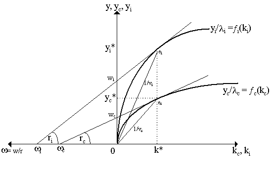
The relationship between the factor intensities of the two sectors and the relative position of the k_c(w) and k_i(w) curves is simple to deduce diagrammatically. Consider Figure 1, where we represent the intensive production functions of the two sectors. Let us begin with a given capital-labor ratio, k*. Suppose we wish to specialize completely in the production of consumer goods, i.e. suppose y_i = 0 so that y = y_c = y_c/l_c, where l_c = 1 (all labor allocated to consumer goods sector) and k_c = k* (so all capital allocated to consumer goods sector). We see immediately that our entire economy is governed by the intensive production function ¦ _c(k_c).

So, with k*, we produce y_c* as our aggregate output. As we know from our discussion of intensive production functions, the slope of the ray tangent to the production function is ¦_c¢ (= r_c), the marginal product of capital, the point where that ray intersects the vertical axis, ¦ _c - k_c¦_c¢ (= w_c), the marginal product of labor. Most importantly, the point where the tangent ray intersects the horizontal axis is w_c = w_c/r_c, the ratio of marginal products. If we specialize in producing consumer goods, then the ratio w_c can be seen as the resulting equilibrium factor price ratio, i.e. the factor prices that clear the capital and labor markets, where the initial supply of capital and labor is captured by the given capital-labor ratio k*.

Now, suppose we specialize completely in investment goods production completely. In this case, y_c = 0, and so y = p·y_i = p·y_i/l _i as l _i = 1 (all labor to investment goods production) and k_i = k* (all capital to investment goods). Thus, aggregate per capita output is governed by the intensive production function ¦_i(k_i) depicted in Figure 1. With the given k*, notice, we will produce y = p·y_i* which (although this depends on p) seems to be more than y_c*. This should alert us to the fact that the investment goods industry is less capital-intensive than the consumer goods industry.

We can see this relative capital intensity diagrammatically in Figure 1 by remembering that the slope of a ray from the origin to the relevant point on an intensive production is 1/v, the reciprocal of the capital-output ratio, v. Thus, letting v_c and v_i denote the capital-output ratios in the consumer goods and investment goods industries respectively, we see immediately in Figure 1 by the rays connecting 0 to e_c and e_i, that 1/v_i > 1/v_c, so that v_c > v_i, in other words, you need more capital per unit of output in the consumer goods industry than in the investment goods industry. Relatively speaking, consumer goods are capital-intensive and investment goods are labor-intensive. Of course, we could have drawn this differently so that the factor-intensities were reversed.

Now, continuing on our specialization into investment goods, we notice that a tangent line with slope ¦_i¢(k_i) intersects the horizontal axis at w _i = w_i/r_i, the equilibrium factor price ratio. Notice immediately that w _i > w _c, which is another indication that the consumer goods industry is relatively capital-intensive. Specifically, note that relative factor shares can be denoted k/w = rK/wL. The higher this k/w ratio, the greater the capital-intensity. In terms of Figure 1, holding k = k* constant, we see that as w _i > w _c, then k*/w _i < k*/w _c, indicating, once again, that the investment goods sector is relatively capital intensive.

Notice the implication of what we have just done: for a given k, the resulting equilibrium factor-price ratio will depend on our allocation between sectors. Specifically, if we allocation all factors to the consumer goods sector, the equilibrium will be w _c; if we allocated all factors into the investment goods sector, the equilibrium will be w_i. The assumption of strict concavity of production functions guarantees this uniqueness. If we do not know the sectoral composition of output, we cannot determine what the actual equilibrium factor-price ratio w is: it can range from a minimum of w _c (complete specialization in consumer goods) to a maximum of w _i (complete specialization in investment goods), i.e. for a given k,

w _min £ w £ w _max

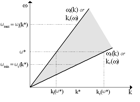
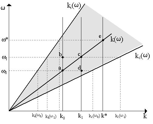
where w _min = w _c and w _max = w _i. The Inada conditions guarantee us that these exist.

Notice also that varying the given k, these upper and lower boundaries for equilibrium factor prices will vary. Specifically, note that in Figure 1, if we increase k above k*, then both w_c and w_i will increase. We depict the resulting boundaries in Figure 2 as the upward-sloping curves w_c(k) and w_i(k). We draw them as straight lines, but this is not necessarily the case. The only things that are posited are (i) that the relationship between k and w _c and w _i is unique and monotonically increasing (by assumptions of strict concavity and constant returns to scale for the production function) and (ii) that the investment goods boundary w_i(k) will always lies above the consumer goods boundary w_c(k) (from the assumption that consumer goods industry is more capital-intensive than the investment goods industry). Naturally, if we change the assumption of factor-intensity, so that investment goods are more capital-intensive than consumer goods, then w_c(k) would lie everywhere above w_i(k).

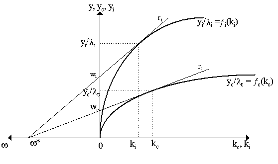
There is, of course, another way of depicting the curves. Specifically, as w_i(k) and w_c(k) are monotonically increasing and unique, then they are invertible, i.e. we can specify the identical curves k_i(w) and k_c(w), where for a given factor price ratio (e.g. w *), we have the resulting capital-labor ratios in both sectors (k_i and k_c respectively). This is identically depicted in Figure 2, but now we read w as the independent variable and k as the dependent..

To see this inversion in production function space, examine Figure 3. The given factor-price ratio w* will set a point on the horizontal axis from which emanate two rays, one with slope r_c and another with slope r_i, corresponding to the marginal products of capital for the consumer goods and investment goods industries. These rays form tangencies with the intensive production functions of both the consumer goods and capital goods industries at points e_c and e_i respectively, which translate into resulting capital-labor ratios k_c and k_i. Thus, this indicates the relationships k_c(w) and k_i(w) that we find depicted in Figure 2. (notice also that k_c > k_i, which is another indicator of the relative factor intensity of the sectors -- use the same formula, k/w , and notice that k_c/w * > k_i/w *).

Notice in Figure 3 that although the factor-price ratio is the same for both sectors, so w * = r_i/w_i = r_c/w_c, we have it that r_i ¹ r_c and w_i ¹ w_c, so it seems that the rates of return to capital and wages are not equal across sectors. But we must not forgot the price of investment goods, p. Specifically, p will be such that p·r_i = r_c and p·w_i = w_c.

Finally, notice that the amount that will be produced when factor prices are w * can be deciphered from y_c/l _c and y_i/l _i on the vertical axes. Notice that both industries have positive output per capita (y_c, y_i > 0), so we are not specializing exclusively in either of them. Both sectors are allowed to operate and the particular amounts they produce will be dictated by the equilibrium factor price ratio we begin with, w *.

This, of course, does not end the story. If we allow both w and k to vary, then the entire shaded region in Figure 2 becomes available as a solution. This is where the rest of the Uzawa model comes into play. Stepping ahead of ourselves a little bit, it might be worthwhile to sketch out what we are aiming for.

We will proceed in reference to Figure 4. Suppose we are given an initial aggregate capital-labor ratio k₀. As we say nothing about allocation between sectors, then there is a whole range of equilibrium factor prices w which are consistent with that allocation (within some maximum/minimum range). Pick one of these factor price ratios. This will then determine a sectoral allocation of k_c(w) and k_i(w). But this may not be necessarily market-clearing, i.e. it may be that l _ck_c(w ) + l _ik_i(w ) ¹ k₀, so that our demands for factors are not equal to our initial supplies of the factor, which implies that the factor price ratio we have chosen is not appropriate. So, for the initial k₀, we must search for a market-clearing factor price ratio that makes demands equal to supplies.

The line k(w) in Figure 4 maps out the locus of equilibrium factor prices for every aggregate capital-labor ratio. The fact that this is upward-sloping everywhere and lies between the boundaries is important. Suppose we begin at k₀. The locus k(w ) tells us that w ₀ is the market-clearing factor price ratio. Thus, the corresponding sectoral allocations k_c(w ₀) and k_i(w ₀) are equilibrium allocations, i.e. l_ck_c(w₀) + l_ik_i(w₀) = k₀. In contrast, for initial capital stock k₀, the wage-profit ratio w ₁ is not market clearing, so l _ck_c(w₁) + l _ik_i(w₁) ¹ k₀. However, for initial capital stock k₁, w₁ is the market-clearing wage-profit ratio (i.e. l _ck_c(w₁) + l _ik_i(w₁) = k₁). So positions a and c represent factor market equilibrium, while positions such as b and d are factor market disequilibrium. The curve k(w) is merely the locus of equilibrium positions.

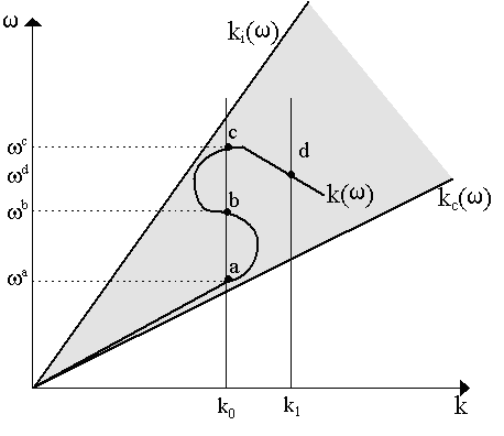
Indeed, all we have been concerned with so far is for an equilibrium at a moment in time -- what the literature calls momentary equilibrium. For obvious reasons, we call this simply a "factor market equilibrium". However, this says nothing about the long-run position of the system. Specifically, any capital-labor ratio k is in factor market equilibrium if we have the right factor prices for it. But a factor market equilibrium does not presuppose or imply steady-state growth.

Suppose (k₀, w₀) is a factor market equilibrium today but it is not a steady-state. Consequently, the production of goods will proceed, and factors will grow at their own rates (labor by the natural rate, n, capital by the sectoral allocation to investment goods production). Nothing we have said so far presupposes that capital and labor will grow at the same rate. Thus, it is likely that tomorrow the capital-labor ratio may be different, say, it may increase from k₀ to k₁. Consequently, tomorrow, new factor equilibrium prices will be obtained (w₁), which determines sectoral allocation, which in turn determines capital growth, etc.

If labor is growing at an exogenous natural growth rate n and we posit some exogenous propensity to save, then (hopefully) there exists a capital-labor ratio k* consistent with steady-state. This is going to be one of the points along the horizontal axis in Figure 4. But, more importantly, as long as our factor equilibrium locus is monotonic, there will be associated with k* is a unique set of "steady-state" equilibrium factor prices, w * and consequently, steady-state sectoral capital-labor ratios k_c(w*) and k_i(w*). If there is not, we have serious problems.

The questions before us are several. Firstly, can we define a factor market equilibrium locus k(w ) that possesses nice properties? By "nice" we mean that it sits "within" the shaded area of Figure 4, and is upward-sloping and monotonic, so that we can define a unique factor price equilibrium w for every aggregate capital-labor ratio k. This is crucial. Suppose not. Suppose we have a situation like the one depicted in Figure 5, where we have a bizarre-looking k(w) locus. For capital-labor ratio k₀, we have three factor market equilibrium prices, w ^a, w ^b and w ^c, which means that from k₀, we are not sure which factor market equilibrium will obtain. As each is associated with a different sectoral allocation (k_c(w ), k_i(w )), we do not know which direction we are heading in!

Let us analyze this troubling case in a bit more detail. As we know, under competitive conditions, r = p·¦_i¢ = ¦_c¢. As a result, we can express p, the price of investment goods in terms of consumer goods, as the ratio of marginal products of capital:

    p = ¦_c¢(k_c)/¦_i¢ (k_i)

Now, as ¦_c¢¢ < 0 and ¦_i¢¢ < 0, then p is proportional to the relative capital-labor ratios k_i/k_c, i.e.

p µ k_i/k_c

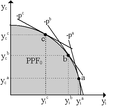
so if k_i is high relative to k_c, then ¦_i¢(k_i) is low relative to ¦_c¢(k_c), which implies that p is relatively high. Thus, the higher k_i/k_c, the higher p will be.

Now, consider Figure 5 again, where we have three factor market equilibrium. Each of these equilibria will be associated with a different price p. So, consider combination a = (k₀, w^a). We can deduce diagrammatically that at this point, k_i/k_c is quite high and thus the corresponding price, call it p^a, will be quite high. Conversely, consider combination c = (k₀, w^c), which has a relatively low k_i/k_c, and thus the corresponding price p^c will be relatively low. So, rather loosely, we can infer that p^a > p^b > p^c.

Plotting the production possibilities frontier associated with k₀ (call it PPF₀) in Figure 6, which plots the feasible combinations of y_c and y_i associated with the capital-labor ratio k₀. We see that the three equilibrium prices p^a, p^b and p^c associated with the respective factor market equilibrium combinations a, b and c in Figure 5 are represented by three price lines with different slopes. In general, as total output is y_c + py_i and k₀ is fixed, then the slope of a price line in PPF space is -p. Recalling that p^a > p^b > p^c, then we see that p^a is the steepest and p^c is the flattest line. All three lines form equilibrium points at their tangency with the PPF, i.e. factor market equilibrium conditions a, b and c in Figure 5 have their corresponding equilibrium output allocations a, b and c in Figure 6.

So, now let us note the following: as p^a is the steepest, then equilibrium a corresponds to an output allocation where the output produced by investment goods sector is relatively high, while the output of the consumer goods sector is relatively low. Conversely, as p^c is the flattest, then at equilibrium c, the output of investment goods relative to consumer goods is small. Thus, factor market equilibrium c corresponds to the least amount of y_i of all the equilibria, while factor market equilibrium a corresponds to the highest amount of y_i of all equilibria.

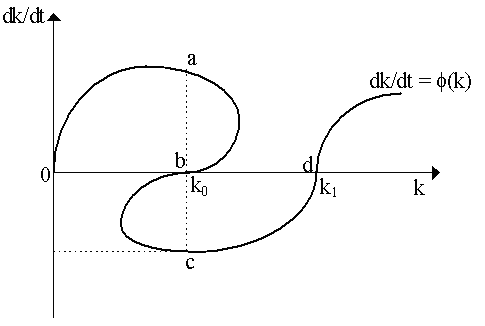
Now, suppose k₀ is a "steady-state" ratio. What does it mean in this context? We have three possible factor-market equilibria associated with it -- and each of them is associated with a different level of investment goods production, y_i. But, recall, g_K = y_i/k₀, so each of these equilibria are associated with different capital growth rates. So if we grant that points a, b and c in Figures 5 and 6 are equilibrium allocations, they surely they cannot all be consistent with steady-state growth!

Suppose that equilibrium b, with investment goods production y_i^b, corresponds to steady-state growth, i.e. y_i^b/k₀ = g_K = g_L. Then, clearly, if we have equilibrium a, then as we see from Figure 6, y_i^a > y_i^b, it must be that g_K > g_L, and so the aggregate capital-labor ratio increases. Thus the combination (k₀, w ^a) cannot be a steady-state. Similarly, if factor market equilibrium c holds, then y_i^c < y_i^b and thus g_K < g_L, so the capital-labor ratio falls and we are not in steady-state either.

Thus, in sum, multiplicity of factor market equilibria at a given aggregate capital-labor ratio k₀ causes real problems. Even if k₀ is a steady-state capital-labor ratio, it is only steady-state if factor equilibrium price w ^b obtains. If, for some reason, the other factor market equilibrium prices w ^a or w ^c happen to hold at k₀, then k₀ is not a steady-state capital-labor ratio.

The implications of this can be understood by examining the resulting differential equation in Figure 7. Notice that at k₀, only equilibrium b corresponds to dk/dt = 0. Equilibrium a corresponds to dk/dt > 0 and equilibrium c corresponds to dk/dt < 0. So, at k₀, we can have steady-state growth, increasing growth or decreasing growth. All three are possible.

A further issue made stark in Figure 7 is that we can also have multiple steady-state capital-labor ratios. There is no reason to assume that k₀ and associated factor market equilibrium b is the only steady-state. A different capital-labor ratio, k₁, with associated factor market equilibrium d can also be a steady-state. The implications for the stability of steady-state are knotty: it could be that some steady-states will be stable, some unstable, some may be only half-stable. In fact, as we shall see later, a differential equation as depicted in Figure 7 can actually yield us a limit cycle, so that we oscillate continuously, but never quite approach a steady-state.

These sorts of trouble will implicate the ability of the economy to approach steady-state growth. We would like to place sufficient restrictions on our model such that most of these difficulties are ruled out. What we want to end up with a k(w ) locus that looks more like the nice, monotonic one in Figure 4 rather than the squiggly one in Figure 5. However, as it turns out, these restrictions are actually quite severe.

So, in sum, the two-sector model poses two essential questions: (1) can we guarantee a unique factor-market equilibrium w for every capital-labor ratio k? (2) is there a unique steady-state growth path k* and can we guarantee that, starting from any capital-labor ratio, the system will approach k* over time? Much of what follows is an attempt to establish sufficient conditions so that we can answer these questions in the affirmative.

Back

Top

Selected References

Next