Incomplete Markets: Existence of Equilibrium

Back

Notation

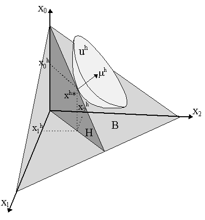
Ignoring the possibility of option completion or dynamic completion, we define a situation of "incomplete asset markets" as when rank(V) < S, i.e. the number of linearly independent securities is less than the number of states. As we have noted earlier, one of the main results of incompleteness is that for any two agents, h, k Î H, we can have it that m _-0^k ¹ m _-0^h for the state multipliers. This "basic property of incomplete markets" implies, then, that we will (probably) not have Pareto-optimality of the resulting allocation. That we still have a resulting allocation is not compromised by the absence of complete markets: agents still have budget constraints and they can still maximize utility accordingly and derive commodity demands and asset demands, etc. and, as a result, obtain a Radner-type equilibrium, albeit one that is not isomorphic to the Arrow-Debreu world.

To understand this, it might be worthwhile to refer to Figure 4. Here we have three states - the initial (0) and two in the future (1 and 2). With complete markets (i.e. two linearly independent assets), a utility-maximizing agent will face a budget constraint such as the (lightly-shaded) pyramid B, thus his can make all sorts of transfers of purchasing power between states. This allows him to attain all sorts of state consumption combinations (x₀, x₁, x₂). Facing such a budget constraint, the agent will choose an allocation which maximizes his utility.

Figure 4 - Restriction of Budget Set with Incomplete Markets

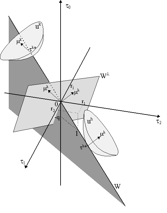
However, if there are incomplete markets, his budget constraint is the (darkly shaded) triangle H in Figure 4. Obviously, H Ì B strictly. Now his possibilities of income transfers across states are severely reduced, but he is still able to maximize his utility. In this case, it would be a point such as x^h* = {x₀^h, x₁^h, x₂^h} in Figure 4, at the tangency of the restricted budget set H and the highest indifference curve, u^h*. m ^h denotes the slope of the indifference curve (or rather, indifference "bowl") at point x^h*. Although he can still maximize his utility and make his choices of consumption/asset demands, would generally be able to achieve a higher degree of utility if the entire budget set B was available to him.

Consider now a similar situation in net transfer space, as in Figure 5. Again, we have the current state (0) and two future states (1, 2). However, we have only one asset, so markets are incomplete and the set of net transfers across states is now restricted to the one-dimensional hyperplane W and the area below it in Figure 5. The slope of W reflects the ratio of the asset price q and the returns in both states, r₁ and r₂ - as shown in Figure 5 by the unit vector 1 on the hyperplane W. Note that if we had complete markets then our hyperplane W would be two-dimensional and we could effectuate all net transfers on or below it. The perpendicular hyperplane W^ is, however, two-dimensional, as shown in Figure 4.

Figure 5 - Equilibrium with Incomplete Markets

In this economy, we have two agents - h and k, both maximizing their utilities subject to the state-transfer constraint, W. Notice that agent h will maximize his utility at t ^h*, thereby achieving utility level u^h* and having state prices m ^h (which are then mapped back to W^ ). In contrast, agent k maximizes her utility at t ^k*, achieving utility level u^k* and state prices m ^k. Notice that m ^h ¹ m ^k, as is obvious from the different slopes of the indifference bowls at t ^h* and t ^k*. This is obvious when we map both state prices back to the perpendicular hyperplane W^ , where we see that m ^h ¹ m ^k again.

Is this an equilibrium? Notice that at t ^h*, t ₀^h < 0 while t ₁^h, t ₂^h > 0, thus agent h is buying the single asset in the initial period in order obtain a return in the future states. In contrast, at t ^k*, we have t ₀^k > 0 and t ₁^k, t ₂^k < 0, thus agent k is short-selling the asset. We have an equilibrium if the amount of the asset demanded by agent h is short-sold by agent k, so that a^h + a^k = 0. Thus, we can still have a Radner-type equilibrium with incomplete markets, just as before, the exception now being that m ^h ¹ m ^k.

Does an equilibrium exist under incomplete markets? Obviously, at this point, we can no longer appeal to equivalence of the equilibrium to the Arrow-Debreu economy. Consequently a new approach must be pursued. Following Magill and Quinzii (1996), we can exploit the Fundamental Theorem of Asset Pricing to this end.  [to be finished later].

Back

Top

Notation

Selected References

Next