|
Attempts at incorporating the foreign sector into the Keynesian model were pursued famously by James Meade (1951) and Jan Tinbergen (1952) - largely in response to the elasticity-absorption debate that was then raging in balance of payments theory. However, the most successful attempt at integrating the foreign sector into the Neo-Keynesian system has been the "Mundell-Fleming Model", the outcome of the research conducted by Robert Mundell (1962, 1963) and J.M. Fleming (1962) while at the International Monetary Fund (IMF). The "Mundell-Fleming" model extends of the IS-LM apparatus to incorporate balance of payments considerations, which has proved quite useful in analyzing international macroeconomic policy. To begin with, let us take the simplest open economy model. In this case, aggregate demand can be defined as:
where NX are net exports (exports minus imports). We can break NX into the following:
where X0 are exports and mY are imports. This form implies that a particular economy's exports are exogenous (X0) but that its imports are a function of its own national income, Y. Note that m is the marginal propensity to import out of income and we assume that 0 < m < 1. We obtain goods market equilibium when aggregate supply meets aggregate demand, Y = Yd or, assuming the simplest consumption function C = C0 + cY, investment function I = I0 + I(r) and assume exogenous government spending G = G0, we obtain in equilibrium:
so exports enter as an autonomous term (X0) whereas the marginal propensity to import is incorporated in the multiplier. In order for this equilibrium to exist, we must assume that 0 < c - m < 1, so that the sum of the marginal propensity to import and the marginal propensity to consume is a fraction. Notice that the open economy multiplier, 1/(1-c-m) is smaller than the closed economy one, 1/(1-c). In relative terms, the IS curve is steeper in an open economy than in a closed economy. However, these relations are far too simplistic: domestic actions, by affecting interest rates, exchange rates and foreign income levels, may affect net exports in more ways. The Mundell-Fleming model incorporates some of these effects into the IS-LM model. Let us define the balance of payments surplus as the sum of the current account surplus and capital account surplus, or:
where NX is the current acount (i.e. net exports) and KA is the capital account (domestic assets owned by foreigners minus foreign assets owned by domestic citizens). If BP > 0 then we have a balance of payments surplus; conversely, if BP < 0 we have a balance of payments deficit. Balance of payments equilibrium is achieved when BP = 0. To enrich the relationships, let us argue that net exports are a function of the real exchange rate, eP/P* where e is the nominal exchange rate (domestic country's currency units per foreign country's currency unit, e.g. dollars per yen), P the domestic price level and P* the foreign/world price level as well as income. Thus we can express net exports as a function:
thus TY < 0 (as income increases, imports increase and thus net exports fall - effectively the same as our previous marginal propensity to import), and dT/d(eP/P*) < 0 (as the real exchange rate rises, net exports fall due to the lower "competitiveness" of exports). Note that the famous "Marshall-Lerner" conditions must be met in order for this last statement to be true. Assuming P, P* are fixed then we can write this relationship simply as NX = T(Y, e). In contrast, the capital account is a function of the difference between domestic interest rates and foreign interest rates, specifically:
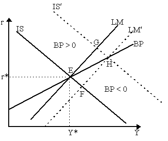
where dk/d(r-r*) > 0 so that if domestic interest rates rise relative to foreign interest rates, then the domestic capital account increases as the greater relative attractiveness of domestic assets implies that domestic and foreign citizens will buy up domestic assets and drop foreign assets. In Figure 8 we have superimposed the external balance locus BP on the IS-LM model. Every point on the BP locus represents a balance of payments equilibrium, BP = 0. Let us assume that exchange rates and price levels are fixed (thus e, P and P* are exogenous) and foreign interest rates are fixed (r* exogenous). Thus, only r and Y are allowed to fluctuate. As a result, a given Y will yield a particular NX whereas a given r will yield a particular KA. So a point on the BP locus is a combination of r and Y that yields BP = NX + KA = 0. The reason for the upward sloping shape of the BP curve is the great advance of Mundell-Fleming model over the older Keynesian model of Meade (1951). Suppose we begin with BP = 0 at some initial Y and r configuration. If Y increases, then NX falls and thus BP < 0. Thus, in order for BP to return to zero, it is necessary for KA to rise - thus domestic interest rates (r) must rise. Thus, there is a positive relationship between Y and r representing the balance of payments equilibrium. The slope of the BP curve is positively related to the marginal propensity to import TY and negatively related to the interest sensitivity of international capital flows, kr. Thus, if there is absolutely no capital mobility (kr = 0), then the BP curve will be completely vertical whereas if there is perfect capital mobility (kr = ¥ ), then the BP curve will be horizontal. Under a fixed exchange rate regime, there is no obvious reason that we will necessarily be at BP = 0. In other words, the IS-LM equations will yield a particular (Y*, r*) that may or may not be where BP = 0. If equilibrium (Y*, r*) is to the right of the BP curve (e.g. at point F in Figure 8), then we have a balance of payments deficit (BP < 0); if (Y*, r*) is to the left of the BP curve (e.g. at point G in Figure 8), then we have a balance of payments surplus. The implications for fiscal and monetary policy are obvious. Beginning at the equilibrium point E in Figure 8 where BP = 0 prevails, we can immediately notice that a monetary policy expansion (a rightward shift in LM to LM¢ ) will yield a new equilibrium F which is below the BP curve, thus we obtain a balance of payments deficit. In other words, from the money supply increase, the consequent rise in Y has driven the current account towards deficit and the fall in r has driven the capital account towards deficit - thus the balance of payments is now in deficit. In contrast, starting from E, a fiscal policy expansion (rightward shift in IS to IS¢ ) will drive the economy to a balance of payments surplus at point G. Here the reasoning is more subtle: the rise in Y has driven the current account towards deficit but the rise in r has driven the capital account towards surplus. The net result depends on the relative slopes of the LM and BP curves. If LM is steeper than BP, then the net result is a balance of payments suplus; if LM is flatter than BP, then the net result is a balance of payments deficit. Thus, the relative sensitivity of international capital flows and income sensitivity of imports are the crucial factors in determining whether an expansionary fiscal policy leads to external deficits or surpluses.
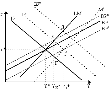
Although fiscal and monetary policy can lead to balance of payments surpluses and deficits, the implication of the Mundell-Fleming model is that one can use a combination of fiscal and monetary policy to increase output without inducing a balance of payments deficit or surplus. This is obvious again in Figure 8 where beginning at E, we can undertake both a fiscal and monetary policy expansions (say, IS to IS¢ and LM to LM¢ ) in such a manner that the resulting equilibrium will be a balance of payments equilibrium (e.g. H in Figure 8). Of course, things are never quite this simple. A balance of payments surplus corresponds to an excess supply of foreign currency which must be bought by the Central Bank; similarly, a balance of payments deficit implies there is an excess demand for foreign currency which must be provided by the Central Bank. However, the Central Bank pays for its purchase of foreign currency with domestic currency and when it sells its foreign currency, it withdraws domestic currency from circulation. Thus, a balance of payments surplus/deficit will increase/decrease the money supply of the economy because the central bank must purchase/sell foreign exchange. As a result, balance of payments surpluses and deficits are not sustainable on their own. For example, suppose there is a monetary policy expansion such that we obtain a balance of payments deficit (as at point F in Figure 8) and thus an excess demand for foreign exchange. The consequent fall in the supply of domestic money as the government sells foreign exchange will gradually shift the LM¢ back to LM and thus equilibrium will return to E. In order to maintain the position at F, the Central Bank must conduct what are known as "sterilization policies". This means that by open market operations or some other domestic tool, the Central Bank increases the domestic money supply exogenously by exactly the same amount as it that money supply was decreased by the foreign exchange sales required to maintain the balance of payments deficit. Thus, the Central Bank "sterilizes" the monetary effects of balance of payments disequilibrium with monetary policy. To sustain a balance of payments surplus, the Central Bank's sterilization policy works in reverse. It is important to note the implications of different policies under different degrees of capital mobility and different exchange rate regimes and sterilization policies. If we maintain the assumption of fixed exchange rates and no sterilization policies, then it is obvious that fiscal policy is more effective than monetary policy. To see this, examine Figure 8 again. Beginning at E, a monetary expansion will shift LM to LM¢ and thus achieve a balance of payments deficit at point F. However, without sterlization, money supply will decline and consequently LM will shift leftwards back to LM and we return from F to E. Thus, monetary policy was completely ineffective at increasing output. In contrast, suppose that, beginning at E, we undertake a fiscal expansion and shift IS to IS¢ and therefore have a balance of payments surplus at point G. Without sterilization, a balance of payments surplus implies that the money supply will increase, therefore shifting LM rightwards to LM¢ . The new equilibrium, at point H, is the resulting long-run position. Thus, output has increased tremendously in this case because the money supply movements in the absence of sterilization reinforce the original fiscal expansion. Thus, under fixed exchange rates, fiscal policy is highly effective and monetary policy is ineffective. Of course, the effectiveness of fiscal policy depends on the degree of capital mobility. If there is no capital mobility so that BP is a vertical line, then notice that both expansionary fiscal and monetary policies are completely ineffective in increasing output. This is because all expansions yield balance of payments deficits and thus lead to reductions in the money supply that bring output back down. In contrast, under perfect capital mobility, when the BP curve is horizontal, monetary policy is again ineffective, but fiscal policy is fully effective, i.e. output rises the full amount of the fiscal expansion as the consequent increase in money supply in the absence of sterilization implies that there will be absolutely no rise in interest rates. We should note here that James Meade (1951) only considered the "no capital mobility" case (vertical BP). Consequently, in order for fiscal or monetary expansion to affect output, Meade argued that the BP locus must be shifted outwards by means of a different and often complicated class of policies seeking to affect net exports, e.g. exchange rate changes, subsidies, quotas, tariffs, etc. The analysis of the impact of such "expenditure-switching" policies were pursued by economists in the 1950s, particularly W.E.G. Salter (1959) and Trevor Swan (1960). It was only in the 1960s, after the arrival of the Mundell-Fleming model which allowed for more capital mobility, that economists realized that internal and external balance could be achieved solely by means of an optimal mix of fiscal and monetary policy without requiring any delicate and complicated expenditure-switching policies. The analysis gets quite different under flexible exchange rates. Recall that if the real exchange rate rises, then NX falls for any level of income. As a result, there are two effects of a rise in exchange rates: the BP curve shifts upwards and the IS curve shifts leftwards. Conversely, a fall in the real exchange rate implies a rise in NX and thus a rightward shift in the BP curve and a rightwward shift in the IS curve. Under a flexible exchange rate regime, there will be none of the rises and falls in money supply due to balance of payments surpluses or deficits. Rather, balance of payments surpluses/deficits result in rises/falls in the real exchange rate and thus movements in the BP and IS curves rather than the LM curve. The implications of flexible exchange rates for fiscal and monetary policies can be visualized in Figure 9. Suppose we begin at E = (r*, Y*) at the intersection of the curves IS, LM and BP and suppose there is a monetary policy expansion from LM to LM¢ . As a result, we move from E to F, where we are in a balance of payments deficit. At F, there is excess demand for foreign currency and excess supply of domestic currency on the foreign exchange market. Under a flexible exchange rate regime, this implies that the real exchange rate will fall, therefore shifting BP rightwards to BP¢ and IS rightwards to IS¢ so that we are now at point J - at a higher equilibrium output level YJ*. Notice that external and internal balance obtain at point J as we have the intersection of IS¢ , LM¢ and BP¢ . Thus, under a flexible exchange rate regime (and unlike a fixed exchange rate regime), monetary policy is quite effective in increasing output.
In contrast, fiscal policy under flexible exchange rates is more ambiguous. In Figure 9, beginning at point E, suppose we have a fiscal policy expansion that drives our IS curve to IS¢ ¢ at point G. However, at point G, we have a balance of payments surplus and thus there will be a rise in the exchange rate which, in turn, shifts BP upwards to BP¢ ¢ and IS backwards from IS¢ ¢ to IS¢ . A new equilibrium is achieved at point K, the intersection of IS¢ , LM and BP¢ ¢ . Obviously, in relative terms, such a fiscal expansion is less powerful under a flexible exchange rate regime than under a fixed exchange rate regime. However, appropriate modifications to this story must be made if fiscal policy expansions lead to balance of payments deficits rather then surpluses (as would result if BP was steeper than the LM curve). In this case, an expansionarly fiscal policy would lead to a deficit and thus a consequent fall in exchange rate, thereby shifting IS and BP outwards. In this particular case, then, the fiscal policy effect on output would be more powerful under a flexible exchange rate regime than under a fixed exchange rate regime. At least until the 1970s, the Mundell-Fleming model remained the tool for the analysis of open economy macroeconomics. Further advances on the Mundell-Fleming framework worth highlighting in addition to Mundell's manifold contributions (cf. Mundell, 1968) are Alexander Swoboda (1972, 1973) on sterilization, W.H. Branson (1974, 1975, 1979) on fuller portfolio and wealth effects and Michael Mussa (1979) on international interdependence and policy coordination. However, just as the closed Keynesian model was challenged by Monetarism during this time, this open Keynesian model was challenged by the "Monetary Approach" to balance of payments equilibrium -- the open economy counterpart of Monetarism. The "Monetary Approach", originally suggested by Frank Hahn (1958) and Robert Mundell (1968) himself, was formalized and popularized by Harry G. Johnson (1972), Jacob A. Frenkel and H.G. Johnson (1978) and Rudiger Dornbusch (1973, 1976). Although Mundell-Fleming and the monetary approach are conflicting in principle, there has been more common ground found between the competing open economy models than in their closed economy counerparts.
|
All rights reserved, Gonçalo L. Fonseca


