|
_________________________________________________________________
_________________________________________________________________ Contents (1) Introduction The "Paretian System" refers to the approach to general equilibrium theory initiated largely by Vilfredo Pareto's Manual of Political Economy (1906). Although often employing tools developed by his predecessors such as Leon Walras (1874), Francis Y. Edgeworth (1881) and Irving Fisher (1892), the hallmark of the Paretian approach is its concentration on agent optimization in a price-taking, multi-market scenario - and thus the emphasis on differentiability and efficiency. The 1930s and 1940s represent the height of the Paretian approach, particularly as channeled through the L.S.E. of Arthur L. Bowley (1924), John Hicks and Roy G.D. Allen (1934), Abba Lerner (1932, 1934, 1944), Nicholas Kaldor (1939), Tibor de Scitovsky (1941, 1942) and, most influentially, through John Hicks's masterpiece, Value and Capital (1939). Elsewhere, the Paretian approach sounded forth in the masterful efforts of Maurice Allais (1943), Oskar Lange (1942) and Paul Samuelson (1947). The basic structure of the Paretian model is similar to the static Walras-Cassel model, although, unlike that construct, everything is now cast in the "tastes-and-obstacles" structure that is the signature of the Paretian system, rather than the "demand-and-supply" functions of the older Lausanne system that the Walras-Cassel model exhibits. As Koopmans was to write many years later:
Perhaps the greatest advantage of the Paretian system is its simple graphical intuition: indifference curves, Edgeworth-Bowley boxes, production possibilities frontiers, community indifference maps, etc. all come together in a simple way to illustrate the conditions for general equilibrium. The great cost is its reliance upon the assumption of differentiability of the various functions employed. The development of the Neo-Walrasian economcs in the postwar period, notably the Arrow-Debreu system of the 1950s, retained the tastes-and-obstacles optimization structure of the Paretian system, but it essentially eschewed its differentiability assumptions and effectively reproduced the same results without it - although the question of whether its reliance on convexity is, in fact, more "general" is a thorny issue. The differentiable approach to general equilibrium lived on largely in international trade theory and only really re-emerged in Neo-Walrasian general equilibrium theory in the 1980s. In the main Paretian model, all agents respond to prices parametically, i.e. they take prices as given, what Pareto (1906: p.115) calls "Type I" behavior. Edgeworth (1881) justified this assumption as a limiting case of a recontracting exchange process when there are an infinite number of agents. Pareto, on the other hand, justified it on the basis of the impossibility of manipulative behavior in a sufficiently complex economy; as he writes:
Households possess factor endowments and desire produced goods for consumption; firms possess nothing, but merely organize production by demanding factors from households and supplying produced goods. The rest of the Paretian system thus follows as in a Walrasian one: given a set of output and factor prices cried out by the "auctioneer", households choose their supplies of factors and demand for goods via a utility-maximization exercise whereas firms decide upon their demand for factors and supply of produced goods via a profit-maximization exercise (as noted, incorporating this last point was one of Pareto's main contributions to the Walrasian system). An equilibrium is then defined as a market-clearing set of prices in both output and factor markets. (2) Graphical Illustration: A two-sector economy Arguably, the greatest advantage of the Paretian system is its intuitive structure and amenability to simple diagrammatic exposition - and thus quite effective as a heuristic device. Graphical illustrations of the Paretian system inevitably require confinement to a simple "two-sector" economy - i.e. an economy with two outputs (and firms), two factors and two households - and thus is quite similar in structure to the "Hecksher-Ohlin" model of international trade. The nomenclature for the two-sector case is then the following:
Agents possess factor endowments and desire outputs. In order to present this diagramatically, we shall ignore factor supply functions and thus assume that agents are "forced" to place all their factors on the marketplace, i.e. K and L are supplied inelastically by agents. As a result, we can capture the consumer's decision as follows. Let UA(XA, YA) is the utility function of agent A which increases with the acquisition of produced goods (XA, YA) and let endowment of agent A be eA = (KA, LA). Obviously, for B, we have UB(XB, YB) and eB = (KB, LB). Together, consumers cannot demand more outputs than are available, thus feasibility requires that:
where X and Y are the total amounts of goods X and Y produced. Utility functions are assumed differentiable. Thus, given prices, pX, pY, r, w, consumer A faces the following optimization problem:
The first order conditions for a maximum are then:
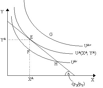
where lA is the Lagrangian multiplier for agent A (or his "marginal utility of income"). Letting UAX = ¶UA/¶XA represent the A's marginal utility of good X and the same for the other goods and factors, then the consumer will choose to demand outputs until:
the ratio of marginal utilities between outputs (also known as the "marginal rate of substitution between X and Y", or simply MRSAXY) is equal to the price ratio, pX/pY. This is the familar condition for a tangency between the budget constraint (with slope equal to - pX/pY and pinned down by the income from the sale of endowments) and the highest indifference curve (with slope equal to - MRSAXY). This is obvious in Figure 1 to be at point E = (XA, YA) which yields utility UA(XA, YA) Bundle G, which yields utility UA¢ ¢ is unattainable given the budget constraint. Conversely, bundles F and H, both of which yield utility UA¢ , are attainable but suboptimal for agent A.
As agent B faces the same problem, then his conclusion will also be that MRSBXY = UBX/UBY = pX/pY at his optimum. Thus, assuming a price-taking economy, as prices faced by agent A and B are the same, then when agents optimize, then it will be true that:
the marginal rates of substitution between the two goods will be the same for both agents. We assume a firm only produces one output, so the production function for the firm that produces good X is X= ¦ X(KX, LX), which says that the output of X is some function (¦ X) of the factors it employs (KX, LX). Similarly, the firm that produces good Y faces the production function Y = ¦ Y(KY, LY) where the output of Y is a function (¦ Y) of the factors it employs (KY, LY). Together, firms cannot employ more factors than are supplied by the agents, thus letting K = KA + KB be the total supply of factor K and L = LA + LB be the total supply of factor L, then the feasibility condition is that:
Each firm attempts to maximize profits subject to given prices factor and output prices. Thus letting p X be the profits of firm X, then the firm's optimization problem is:
and the same applies for firm Y if we replace X with Y. Assuming the production functions are differentiable, then the first order conditions for a maximum are:
Letting ¦XK = (¶¦X/¶K) and ¦XL = (¶¦X/¶L) be the marginal physical products of K and L respectively, then the firm will employ factors (and thus produce output X) until:
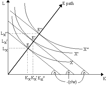
i.e. the ratio of marginal products is equal to the factor price ratio. The ratio of marginal products is also known as firm X's "marginal rate of technical substitution" between K and L, or MRTSXKL = ¦ XK/¦ XL. The MRTSXKL is the slope of the firm's isoquant, thus this condition claims that the firm will hire factors (and thus produce) until where the slope of its isoquant is tangent to the isocost line - once we fix one. We can see this diagramatically below in Figure 2. A given factor price ratio (r/w), will determine an entire series of isocost lines. At any isocost line, the firm will maximize profits by choosing input combinations (KX, LX) and level of output (X) such that the slope of the isoquant (= MRTSXKL) is equal to the slope of the isocost line (r/w). Thus, in our diagram, points E, E¢ and E¢ ¢ all represent profit-maximizing choices of inputs and output levels that maximize profits given different isocost lines. The thick line passing through E, E¢ and E¢ ¢ , denoted "E path", represents firm X's "output expansion path" given r/w and, in this diagram, its constant slope indicates that the firm's technology exhibits homotheticity (e.g. the production function is homogeneous of some degree).
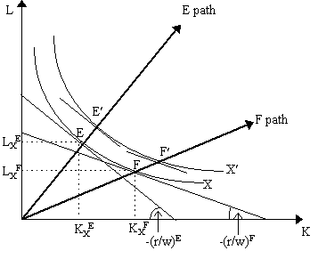
If r/w was different, we would have a different output expansion path. For instance, if r/w was lower, then our first order conditions tell us that firm X would employ more K relative to L. We can see this in Figure 3 where we compare (r/w)E > (r/w)F. At a particular level of output X, we can see that the optimal input combination for factor returns (r/w)E is given by KXE and LXE and for factor returns (r/w)F, we have KXF and LXF. Thus, as r/w falls, the optimal input combination for a given X involves an increase in K and a fall in L. By homogeneity of whatever degree of the production function, this would be true at every level of output, e.g. X and X¢ , thus we could draw two output expansion paths, the E path and the F path, corresponding to different levels of X where the E path refers to factor returns (r/w)E and the F path refers to the lower factor returns (r/w)F.
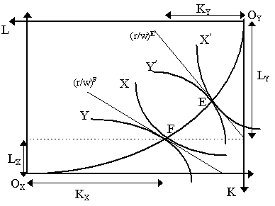
Nonetheless, at a given r/w, in order to obtain the precise input combinations that firm X produces it is thus necessary to either fix total costs and have the firm maximize output or set a particular output level and permit the firm to minimize costs. The interesting question that emerges is what will be the levels of KX, LX and X that the firm chooses when maximizing profit for a given px and r/w if we do not arbitrarily pin down a particular cost level or output level? In fact, if we consider firm X in isolation, we cannot pin these down at all unless we assume ideas about Marshallian increasing costs/diminishing returns via factors specific to the firm - which, as Piero Sraffa (1926) has shown, are nonsensical for a single firm in a perfectly competitive economy. What is necessary, as insinuated by Sraffa, is to consider the firm in a general equilibrium framework as that will provide the necessary "increasing cost" properties that permit us to pin down the levels of output and inputs demanded in each industry. (see our survey of production theory for more details.) To understand this, recall that value, as the more faithful Neoclassical economists (e.g. Wieser, 1889, Knight, 1928; Robbins, 1934), insisted repeatedly, arises solely from opportunity cost and opportunity cost will not arise unless there is scarcity, i.e. there are fixed supplies of resources upon which demands are made. In this context, this means that we cannot consider the firm in isolation and hope to determine what KX, LX and X will be as we cannot restrict costs or outputs arbitrarily. We must consider what the impact its output and factor demand decisions will be on other firms. The greater the output of firm X, the more resources it will require and thus the less available to firm Y. Such a notion, of course, may conflict with the idea of perfect competition as the increase in output of a firm will influence not only its own cost conditions but also those of other firms, and in a two-sector model such in inevitable, but we have so far considered X as a single firm. There is no reason not to assume that it is instead an aggregate of "perfectly competitive" firms producing output X, arbitrarily divided. The basic notion, then, is that as long as there is an inelastic supply of factors and all are fully employed, then for the output of X to rise, factors must be released from firm Y and thus the output of firm Y must fall. However, unless both X and Y use effectively the same technology, the amount of factors released by a reduction in output of industry Y will be of a different proportion to the absorption requirements of industry X. Hence, an increase in the output of industry X requires an increase in demand for K and L which is different from the factors released by a decline in output of industry Y. As a result, the factor which industry X uses more intensively will rise in price relative to the factor it uses less intensively. As Joan Robinson put it, "for any commodity considered separately, .... an increase in the output of any commodity turns the relative factor prices against itself." (J. Robinson, 1941). This process can be understood by using an Edgeworth-Bowley box for production, as in Figure 4. Total factor supplies K and L set the size of the box. A particular point in the box represents an allocation of resources K and L between the different industries, X and Y. Notice that full employment is assumed, thus at an allocation point such as F, industry X employs LX and KX and industry Y employs KY and LY and, by the full emploment assumption, KX + KY = K and LX + LY = L. Seeing the bottom left and the upper right corners of the box as the origins of an isoquant map for industries X and Y respectively, we can thus figure out the levels of output in each industry which correspond to allocation F. [Historical note: the misnamed box as drawn here was first introduced by Pareto (1906: p.138) and is only implicit in Edgeworth (1881: p.28) and drawn differently in Bowley (1924: p.5). Although Allais (1989: p.67, 620), defying "intellectual gangsterism", has reverted to calling it a "Pareto box", we shall sheepishly retain its conventional usage.]
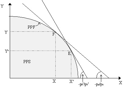
The curved line connecting OX and OY represents the "contract curve" between industries X and Y which represents the set of allocations where the isoquants of each industry are tangent to each other. In this particular diagram we assume that industry X is more intensive in K and less intensive in L relative to industy Y. Thus, starting from the origin OX, we can see that as output of industry X rises that of industry Y falls, then industry X is "turning" the factor prices against itself. In other words, as X increases from, say, X to X¢ , then factor returns rise from (r/w)F to (r/w)E - and thus firm X will choose a different input combination. In terms of our earlier Figure 3, think of firm X being shunted from the F path to the E path as output climbs from X to X¢ and factor prices increase from (r/w)F to (r/w)E. In this sense, as we increase the output of industry X and decrease the output of industry Y, then output expansion rays from OX rotate counterclockwise for X. Thus, unlike the consumption case, in a production Edgeworth-Bowley box, the contract curve connecting OX and OY has a precise, curved shape of Figure 4 reflecting different factor intensities in both industries. If we drew a diagonal line from OX to OY, then, save for the origins, the contract curve would lie completely to one side of it. Notice that, in contrast, if X were relatively more intensive in L than X, then the curvature of the contract curve would be reversed and it would lie on the other side of the box so that as X rises, the output expansion rays from OX would rotate clockwise. We can represent the locus of tangencies in Figure 4, the contract curve, as a "production possibilities frontier" (PPF) or "transformation surface" as depicted in Figure 5, first introduced by Abba Lerner (1932) and Gottfried Haberler (1933: p.176). What may be called the production possibilities set (PPS) is the area below the PPF curve and above the axes. The PPF represents the trade-offs between outputs X and Y. As output X increases, output Y decreases, etc. In Figure 5, points E and F represent output combinations equivalent to those in Figure 4. Notice that the curvature of X and Y represents not diminishing returns or any Marshallian paraphenelia (recall both our industries have constant returns to scale), but rather the different relative factor proportions which each industry uses, the "turning" of factor prices against one's self as factors are released from one industry to another. The PPF would be linear only if industries X and Y had the same relative technology and thus each industry absorbs factors in exactly the same proportion as they are released by the other industry.
It is a simple matter to notice that the (negative of the) slope of the PPF is merely the "marginal rate of product transformation" betwen outputs X and Y (also known as MRPTXY). Notice that as we increase output of good X and decrease output of good Y, then, at the margin, we release dL from Y to X, then output of X increases by dX = ¦XLdL while output of Y falls, or -dY = ¦YLdL. Thus, combining these two via dL, we obtain the result that
Thus, the negative of the slope of the PPF is merely the ratio of the marginal products of labor in each industry, ¦YL/¦XL. This ratio is the marginal rate of product transformation (MRPTXY). If we had released K instead by marginal amount dK, then we would obtain the result that -dY/dX = ¦YK/¦XK. Thus, it must be that
By cross-multiplying, we can rewrite this last equality as:
which simply states the familiar condition that MRSXKL = MRSYKL, the marginal rates of substitution in both industries are equal - the condition implied by the tangency of the isoquants in the Edgeworth-Bowley box in Figure 4. Thus, a point on the PPF in Figure 5 indeed represents points on the contract curve in Figure 4. However, we can say something more. The production possibilities frontier in Figure 5 permits one to connect output prices (pX, pY) and factor prices (r, w). Recall from the first order conditions for profit maximization for firm X we obtained the result that w = pX¦XL and for firm Y we obtained w = pY¦YL, thus combining:
As MRPTXY = ¦ YL/¦ XL, then this is equivalent to stating that:
Thus, drawing a price line (as in Figure 5) with slope equal to the (negative of) output prices, pX/pY, we obtain that the only point on the PPF where px/pY = MRPTXY (i.e. the price line and PPF are tangent) is at point F. Thus, only output combination X and Y are consistent with profit-maximization. A different price ratio (noted as pX¢ /pY¢ in Figure 5), would be tangent to the PPF at point E, thus E would be the only output combination (noted here X¢ and Y¢ ) which is consistent with profit-maximization. Additionally, note that the marginal cost of increasing output by firm X is merely w/¦ XL while the marginal cost of increasing output by firm Y is w/¦ YL. Thus, when we can rewrite the profit-maximizing condition as:
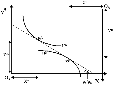
which effectively yields two things: (i) that MRPTXY can be regarded as the ratio of marginal costs for each firm; (ii) that the profit maximization exercise implies that output price equals marginal cost of output for each firm, i.e. pX = w/¦XL and pY = w/¦YL. Finally, note that the second order condition for profit-maximization implies that for firm X, pX¦XLL £ 0, px¦XKK £ 0 and ¦XKK¦XLL - ¦XKL¦XLK ³ 0. This implies that the production function for firm X, ¦X(K, L) must be concave in the neighborhood of the maximum. As a result, a maximum cannot be achieved where the marginal products of both inputs are increasing locally, i.e. we cannot allow for local increasing returns to scale. Translated to the PPF world, the implication is that we cannot have non-convexities in the production possibilities set. From these exercises, we can immediately begin to see the "imputation" idea of Friedrich von Wieser (1889) in this context. Given output prices, we can "impute" what the corresponding factor prices have to be. Namely, given pX/pY, we know that output has to be (X, Y) in Figure 5, and we can then translate this, via the corresponding point F in the Edgeworth-Bowley Box in Figure 4, we can notice that the factor returns ratio has to be (r/w). If we are given different output prices (pX¢ /pY¢ ), then we know output has to be X¢ , Y¢ and thus, via point E, we know that the factor returns ratio has to be (r/w)¢ . Thus, by merely knowing output prices, we can then determine outputs, factor prices and factor employments in different industries. However, there are two exogenous elements here: the supply of factors and output prices - exactly like in the linear Walras-Cassel model. Once we know these, the rest (output produced, factors employed and factor prices) follows. One ought then to suspect that, like the Walras-Cassel model, the supply of factors and output prices both emerge from the household utility-maximization exercise. We presumed, for purposes of graphical presentation, that households supply factors inelastically, but it would not be difficult to notice that if we allow household factor supplies to vary, we would be varying the size of the Edgeworth-Box and the PPF. What about output prices? In principle, households take these as given and then, via utility-maximization, we obtain demands for commodities. However, suppose that given certain output prices, the corresponding household demands for commodities are not equivalent to the output of commodities that are implied by the same price ratio operating on the PPF? In this case, we cannot say we have an "equilibrium". For an equilibrium, the outputs demanded must equal the outputs supplied - and, hopefully, there is such a price ratio. To see this in diagrammatic form, we need only consider the issue of allocation of output. Given output prices pX and pY, we obtain a given amount of commodities produced X and Y. These will form the dimensions of a consumer Edgeworth-Bowley box as depicted in Figure 6. As a particular output price ratio determines r/w, and as we are assuming supply of factors are supplied exogenously, we can pin down the income of each household A and B as mA = rKA + wLA and mB = rKB + wLB. As we are given pX/pY, then each household will maximize utility subject to such a constraint. We have an equilibrium if the resulting demands are equal to output. In Figure 6, as we can immediately see visually, this is indeed not the case as we have an excess supply of good X (as XA + XB < X) and an excess demand for good Y (as YA + YB > Y).
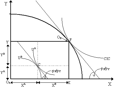
Consequently, we have an equilibrium only if the output prices are such that maximizing utility, the sum of demands of both housholds will be equal to the amount supplied by firms. This will only be true if the indifference curves are at a tangency to each other. This is visualized in Figure 7 where we have fitted a consumer Edgeworth-Bowley Box within the Production Possibilities Frontier by taking our origin the origin of the diagram as the origin of consumer A (OA) and point F as the origin of consumer B (OB). At equilibrium prices, pX/pY, we can define X and Y as the profit-maximizing point F on the PPF. At that same output price ratio, pX/pY, within the consumer Edgeworth-Bowley box, indifference curves of agents A and B are tangent to each other at point C. At that tangency, the outputs demanded by households are XA + XB = X (thus the market for X clears) and YA + YB = Y (thus the market for Y clears).
We achieve a general equilibrium if all markets clear - which means that output prices and factor prices are such that the demand for each factor equals the supply of each factor and the demand for each good equals the supply of each good, i.e. there is a set of prices (pX, pY, r, w) such that:
where (XA, YA), (XB, YB) satisfy the consumers' utility-maximzation exercise and (KX, LX), (KY, LY) satisfy the producers' profit-maximization exercise. Is there such a set of prices? The early employers of this model did not answer this question satisfactorily. Rather, they proceeded to count equations and unknowns and, once these were found to be equal, were satisfied that a solution existed. The situation depicted in Figure 7 represents a general equilibrium situation because all of the following hold:
As a consequence, it is obvious that the conditions for an equilibrium are that:
All these conditions are obvious. The last is the condition that the pX/pY which is tangent to the PPF is the same as the pX/pY that is in the interior of the Edgeworth-Bowley box forming the tangency to the households's indifference curves, thus MRSXYA = MRPTXY. We can see this last point more clearly by constructing a "community indifference curve" (CIC) which has the same slope at F on the PPF, as the consumers have at point C in the interior of the box. The third condition, then, can be represented by saying that the slope of the community indifference curve (CIC) must be equal to the PPF. We shall postpone the construction of the CIC until later, when we consider welfare theory more carefully. The structure of the two-sector model can be expanded into a multi-sectoral model where we have m factors, n goods, F firms and H households. In this case, we do not need to place any arbitrary restrictions: we allow firms to produce several outputs, for instance, and allow households to possess a factor supply function which arises from utility-maximization rather than imposing that these be supplied inelastically. Furthermore, we shall allow households to own shares of firms, thus their income is no longer confined to the sale of endowment but also to the profit shares they own. Of course, with all this, the model is no longer amenable to diagrammatic representation, but similar conclusions can effectively be reached. Our primary task is to tackle the issue of the existence of an equilibrium in a multi-sectoral model. Like Walras (1874), Vilfredo Pareto (1906: p.446-8; 482-3) was content to count equations and unknowns to establish the existence of an equilibrium. Given the resemblance of the Paretian structure to the Walras-Cassel structure, we shall attempt to maintain more or less the same notation we had before. The notation and environment is as follows:
To ease notation, we assume that all price vectors are row vectors and all quantity vectors are column vectors. We also assume, for simplicity, that there are no intermediate goods, thus firms do not demand produced goods. Each firm f = 1, .., F has a production function (technology) represented by the implicit function F f(xf, vf) = 0 which transforms factors demanded (vf) into outputs supplied (xf) by the fth firm. It is assumed that output increases and inputs increase. Firms seek to maximize profits, thus the fth firm's profit (pf) arises from the difference between total revenue from the sale of commodities (pxf) and total costs from factor payments (wvf). Thus, the fth firm has the following optimization problem:
As there are F firms, there are F such profit-maximizing programs. Profits obtained by firms are distributed to households as profit income. Thus, letting qhf denote the hth household's share of firm f's profits, then a fully privately owned economy implies that we can normalize profit shares as å h=1H q hf = 1, i.e. the sum of firm f's shares is equal to one. It is assmed that profit shares are not unknowns in this economy, but rather are given as data. We assume each household h = 1, ..., H has a utility function (Uh) representing preferences and a particular endowment of factors, only vh of which is supplied to the economy. Utility of the hth household is a function of outputs consumed (xh) and factors supplied (vh) - increasing with the former and decreasing with the latter. Thus, households seek to maximize Uh(xh, vh). Households obtain income from the sale of factors (wvh) and the profit shares (qh p ) where q h = [q hf]f=1F is the vector of shares owned by the hth households (i.e. qh is household h's "portfolio") and p = [pf]f=1F is the vector of firms' profits. It uses the proceeds from factor sales and profit shares to demand produced commodities, thus total purchases of household h, pxh cannot exceed income (wvh + qh p ). The hth household's utility maximization problem is then:
As there are H households, there are H such optimization programs. Let us now establish the number of equations. From the H utility maximization and F profit-maximization problems we obtain the following first order conditions (note: m h is the Lagrangian multiplier for the hth household; m f is the Lagrangian multiplier for the fth firm). From the household's optimization problem we obtain the following: (1) ¶Uh/¶xih = mhpi for i = 1, .., n; h = 1, .., H. as we have n commodities and H households, we have nH such equations (one per commodity per household). (2) ¶Uh/¶vjh = - mhwj for j = 1, .., m; h = 1, .., H. as we have m commodities and H households, we have mH such equations (one per factor per household). (3) pxh = wvh + q h p for h = 1, .., H we have H budget constraint equations (one per household). From the firms' optimization problem, we obtain the following first-order conditions: (4) pi = -mf (¶Ff/¶xif) for i = 1, .., n; f = 1, .., F. as we have n commodities and F firms, we have nF such equations (one per commodity per firm) (5) wj = mf (¶Ff/¶vjf) for j = 1, .., m; f = 1, .., F. as we have m factors and F firms, we have mF such equations (one per factor per firm) (6) Ff(xf, vf) = 0 for f = 1, ..., F. we have F such equations (one per firm) We now have to impose market-clearing for equilibrium. Thus: (7) å h=1H xih = å f=1F xif for i = 1, .., n is the market clearing condition for commodity i. We have n commodities, thus we have n such equations (one per commodity). (8) å h=1H vjh = å f=1F vjf for j = 1, .., m is the market clearing condition for factor j. We have m factors, thus we have m such equations (one per factor). Thus, adding up, we obtain the following:
We can remove one equation by Walras's Law. Summing up budget constraints over households and recognizing that the profits shares for a particular firm f equate to one and then plugging in firms' profits yields, after some rearrangement: (9) å i=1n pi [å h=1H xih - å f=1F xif] + å j=1m wj [å f=1F vjf - å h=1H vjh] = 0 or, in vector form:
which is the familiar statement of Walras's Law. Note that if all markets clear but one, then that last one will necessarily clear too. Thus, we can exclude one of the market-clearing conditions from our list. Thus, now, the number of equations becomes:
Let us now turn to the establishing the number of unknowns. From household h's optimization problem, the unknowns are xih for each good i = 1,.., n; vjh for each factor j = 1, .., m and m h (Lagrangian multiplier from utility-maximization), thus for each household we have n+m+1 unknowns. As we have H households, then we have (n + m + 1)H unknowns from the household side. From firm f's optimization problem, unknowns are xif for each good i =1,.., n; vjf for each factor j = 1, .., m and m f (Lagrangian multiplier from profit-maximization), thus for each firm we have n + m + 1 unknowns. As we have F firms, then we have (n+m+1)F unknowns from the firm side. From the market-clearing situations, we have pi from every commodity market, i = 1, .., n and wj for every factor market j = 1, .., m, thus we have n + m unknowns. Thus, for the entire system we have:
It seems to exceed equations, but we forgot the numeraire good. We can thus set, say, the price of the first commodity to one (i.e. p1 = 1) and so one of the unknowns drops out. Thus total unknowns are now:
Thus, in conclusion, the total number of equations is equal to the total number of unknowns. Pareto (1906) concluded that this was enough to establish the existence of a general equilibrium for the economy. (On to the Paretian System II: Efficiency) _________________________________________________________________ Maurice Allais (1943) Traité d'Économie Pure, 1952 edition of Á la Recherche d'une Discipline Économique, Paris: Impremerie Internationale. Francis M. Bator (1957) "The Simple Analytics of Welfare Maximization", American Economic Review, Vol. 47, p.22-59. Gottfried von Haberler (1933) The Theory of International Trade: with its applications to commercial policy. 1937 translation, New York: Macmillan. John Hicks (1939) Value and Capital: An inquiry into some fundamental principles of economic theory. 1946 Edition, Oxford: Clarendon Press. Frank H. Knight (1928) "A Suggestion for Simplifying the Statement of the General Theory of Price", Journal of Political Economy, Vol. 36 (3), p.353-70. Oskar Lange (1942) "The Foundations of Welfare Economics", Econometrica, Vol. 10 (3), p.215-28. Abba P. Lerner (1932) "The Diagrammatical Representation of Cost Conditions in International Trade", Economica, Vol. 12, p.346-56. Abba P. Lerner (1934) "The Concept of Monopoly and the Measurement of Monopoly Power", Review of Economic Studies Abba P. Lerner (1944) The Economics of Control: Principles of welfare economics. New York: Macmillan. Vilfredo Pareto (1906) Manual of Political Economy. 1971 translation of 1927 edition, New York: Augustus M. Kelley. Lionel C. Robbins (1934) "Remarks upon Certain Aspects of the Theory of Costs", Economic Journal, Vol. 44, p.1-18. Joan Robinson (1941) "Rising Supply Price", Economica, Vol. 8, p.1-8. Paul A. Samuelson (1947) Foundations of Economic Analysis. 1983 edition. Cambridge, Mass: Harvard University Press. Tibor Scitovsky (1941) "A Note on Welfare Propositions in Economics", Review of Economic Studies, Vol. 9, p.77-88. Tibor Scitovsky (1942) "A Reconsideration of the Theory of Tariffs", Review of Economic Studies, Vol. 9, p.89-110. Friedrich von Wieser (1889) Natural Value. 1971 reprint of 1893 translation, New York: Augustus M. Kelley. _________________________________________________________________
|
All rights reserved, Gonçalo L. Fonseca
