|
Notation One of the central features of sequence economies are financial markets. Before proceeding onto defining a full sequential equilibria, it might be worthwhile to spend a few moments concentrating on financial asset market equilibrium. An asset is a financial instrument which carries a current purchase price and a future payoff -- or, rather, an entire series of future payoffs depending on the states that emerge in the future. The simplest kind of asset is a bond, which pays a sure monetary payoff in the future regardless of the state that actually occurs in the future (net of default risk). With stocks, of course, the payoff is not certain and depends on corporate profits which will in turn depend on the state of nature that emerges in the future. Other assets, of course, have different payoff structures. Nonetheless, despite these differences in detail, in general, financial assets are transfers of purchasing power across time periods and states of nature. Buying an asset implies we are transferring purchasing power from the present to some future state; selling or short-selling an asset implies we are transferring purchasing power from some future state to the present. Regardless of the type of financial asset - stocks, bonds, options, etc. - all of them involve at least these time-and-state spanning properties. An asset market is, naturally, the "place" where assets are traded and, consequently, purchase prices are determined. The determination of asset prices is one of the main concerns of financial theory and there are a handful of competing theories. However, one of the central features of asset pricing theory, or, as some claim, "the one concept that unifies all of finance" (Dybvig and Ross, 1987), is the stipulation that, in equilibrium, asset prices are such that "arbitrage" is not possible. It might be useful to clarify at this point what is meant by "arbitrage". Intuitively, many people would associate arbitrage with "buying low and selling high". More formally, an arbitrageur purchases a set of financial assets at a low price and sells them at a high price simultaneously. This timing element is important: namely, because of simultaneity, arbitrageurs require no outlay of personal endowment but only need to set up a set of simultaneous contracts such that the revenue generated from the selling contract pays off the costs of the buying contract, i.e. construct a portfolio consisting of purchased assets and short-sold assets which yields positive returns with no commitment. The simultaneity ensures that the arbitrageur carries no risk as none of his own personal resources are ever on the line. One can argue that, in the "real" world, there is rarely a case of pure arbitrage. Indeed, most of what the financial community calls "arbitrage" is really just some very fast or short-term speculation. When speculating, agents usually purchase the assets first and sell them afterwards (or short-sell the assets first and purchase them afterwards), thus they must commit some of their own resources, at least temporarily -- and they still run the risk that they will not get to dispose of the second half of their operation at the anticipated price. Pure arbitrage, in contrast, is simultaneous and riskless - the quintessential "free lunch". The reason why pure arbitrage is not commonly observed is precisely the reasoning for the "no-arbitrage" assumption in financial market equilibrium: if there were arbitrage opportunities, these would be eliminated immediately. Specifically, if asset prices allow for arbitrage opportunities, then because of strong monotonicity of preferences and no bounds to short-selling, agents would immediately hone in on a portfolio position that yielded arbitrage profits. The "no-commitment" nature of arbitrage opportunities imply that agents can replicate this arbitrage portfolio infinitely with no personal resource constraint. If this begins to happen, then at some point (i.e. almost instantly), the price differences which enabled the arbitrageur to hold such a position would close. Thus:
The concept of no-arbitrage asset prices in financial theory stretches over naturally into sequential general equilibrium theory where asset market equilibrium is part of the structure. In order to visualize this, let us begin with the simplest model possible. Suppose we have a two-period economy with T = (0, 1) with one (consumption) good and one financial asset which yields a known, riskless return (say, a bond). Let H be the set of consumers, where, abusing notation, #H = H. Each agent h Î H has an endowment of the consumption good in each of the two periods, eh = {e0h, e1h} and has preferences ³ h defined over the amount of the consumption good consumed each period. Thus, an agent can receive a bundle xh = {x0h, x1h} Î R2+ denoting the amount of consumption good he consumes in period 0 and 1 respectively. As preferences ³ h are defined over R2+, then with enough assumptions, we can define a nice utility function uh: R2+ ® R with all the desirable properties. Let p = {p0, p1} denote the prices for the consumer good in periods 0 and 1 respectively (superfluous in this simple one-good example, but we shall maintain them nonetheless). The consumer can purchase some amount ah of the asset in period t = 0. A unit of the asset can be bought at price q in period t = 0 and will yield a return r in period t = 1 (formally, the return to an asset is defined as the final payoff divided by the initial price, but we shall jump straight into returns here). Thus, the consumer wishes to fulfill the following program:
thus, he chooses a consumption plan xh* = (x0h*, x1h*) and the amount of the asset to purchase ah*. Note that that ah can be positive or negative: if ah > 0, then the agent is buying an asset, in which case he must surrender qah at t = 0 in order to gain rah at t = 1. If ah < 0 then he is "short-selling" an asset, in which case he is receiving qah at t = 0 but must pay rah at t = 1. Note that this model is basically the same in structure as that of Irving Fisher's (1930) famous two-period model - and thus its solution is too well-known to be worth mulling over. Nonetheless, it can be used to obtain a intuitive understanding of the meaning of arbitrage-free prices and asset market equilibrium. The first step is to define an arbitrage opportunity which can be stated in this simple context as follows:
The principle distinction is that arbitrage of the first kind guarantees positive returns with non-positive commitments (think of borrowing and lending at different rates) whereas the second kind guarantees non-negative returns with negative commitments (a "free lunch"). Thus, in an arbitrage opportunity of the first kind, qah £ 0, thus the agent is not buying any asset at time t = 0, thus makes "no commitment", or outlays none of his endowment at time t = 0 to purchase assets (although he can sell assets). However, notice that while although he has sacrificed no endowment, he is nonetheless making a positive return in the future, rah > 0. In an arbitrage opportunity of the second kind, qah < 0, he is short-selling the asset and thus has "negative commitments", i.e. he is increasing his "endowment" or purchasing power in period t = 0. However, in this case, rah ³ 0, i.e. he makes no future payments and possibly even makes positive gains. Thus an arbitrage opportunity in general can be thought of as a series of trades where an agent commits none of his own endowment and yet makes positive gains along the line. Thus, we can define a "no arbitrage" or "arbitrage free" asset price q as follows (using the definition of arbitrage of the first kind):
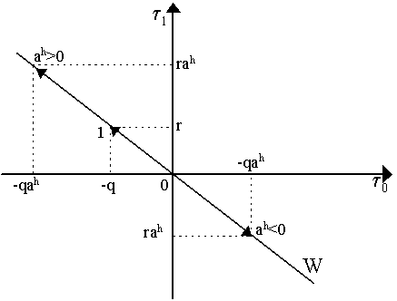
i.e. there is no portfolio ah such that an agent can make a non-positive commitment (qah £ 0) that yields a positive return (rah > 0). In Figure 2, we can see the meaning of this quite clearly in a net trade diagram for the hth household. Let t 0 denote net trades in the initial period (t = 0) and t 1 denote net trades in the future period (t = 1). Thus, a particular net allocation t = (t 0, t 1) exchanges some amount of the current consumption for future return or vice-versa, i.e. t 0 = p0(x0 - e0) and t 1 = p1(x1 - e1) (again, we could drop consumer goods prices out if we wished). The origin (t 0 = 0, t 1 = 0) represents the situation where the agent consumes his endowment in each period and makes no intertemporal trades (i.e. neither purchases nor sells assets). If the agent purchases merely a single unit of the bond, denoted as 1 in Figure 2, then he must pay q and gets r in the future state, thus his net trades are t 0 = -q and t 1 = r. As ah is the number of bonds an agent purchases or short-sells, then if he buys ah bonds, his net trades are t 0 = -qah and t 1 = rah. Let us define the following:
Thus, W is a line (or hyperplane) in R2 that passes through the point (-q, r) which we have labeled 1 to represent a unit of the bond. As -q and r are given, then the slope of the hyperplane is constant at -r/q and passes through the origin. As noted, if ah > 0 then he is buying bonds, so that t = (-qah, rah) lies on the hyperplane W in the northwest quadrant. If ah < 0, then he is short-selling bonds so that t = (-qah, rah) lies on the hyperplane in the southeast quadrant Finally, if ah = 0 (so t is at the origin), the agent is not doing either. For the moment, there are no upper or lower limits on the amount of assets purchased or short-sold. Notice that in our diagram, as W passes through the origin, then -qah+ rah = 0 for all ah Î R, thus current commitments (-qah) are equal to future gains (rah). Consequently, any point on the hyperplane W or below it represents a situation of no arbitrage as defined above.
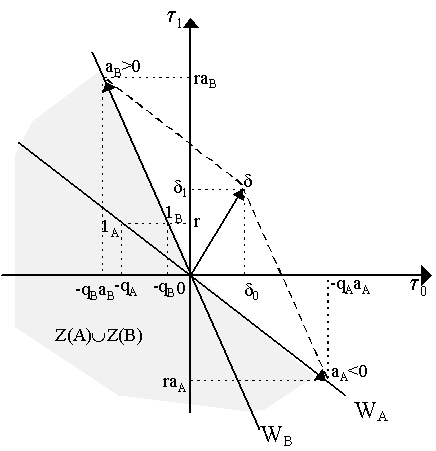
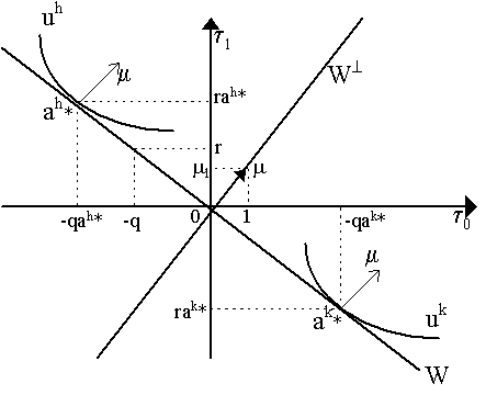
No Arbitrage Opportunities How might we represent a situation with arbitrage opportunities? This is shown in Figure 3. Let us suppose that we have two issuers of bonds, say A and B so that returns on each of the bonds they issue are the same (rA = rB = r) but their respective purchase prices is different (thus qA ¹ qB). Letting qA > qB, then our diagram changes so we now have two hyperplanes WA and WB (Figure 3). Notice that 1A and 1B represent the purchase of a unit of the bond issued by A and the bond issued by B respectively. Now, as both WA and WB go through the origin, it may seem as both qA and qB are "arbitrage free". Individually this is true: we cannot buy and sell a single asset (say asset A) and make arbitrage gains. However, considered together, we do have an arbitrage opportunity immediately available to an arbitrageur. To see this, suppose an agent short-sells the high-priced bonds (i.e. bond A) by the amount aA (< 0) so that he gains -qAaA. He can use part of the proceeds of this short-sale to purchase amount aB of the low-priced bond B, thus outlaying -qBaB. We can see, diagramatically in Figure 3, the consequences of such a procedure: namely, the "net gains" of the arbitrageur are d 0 = (-qAaA) - (-qBaB) > 0 and d 1 = r(aB + aA) > 0 and thus net gain vector d = d 0 + d 1 lies in the positive orthant of R2. Of course, the agent need not limit himself to merely selling aA and purchasing aB but, as long as the prices qA and qB are fixed and bonds of each type are supplied without end by the market (i.e. "perfect competition"), then the arbitrageur can do infinite amounts of such operations and thus increase his arbitrage gains to infinity. Arbitrage Opportunities What enables this to happen? Namely, there is a "non-convexity" which is occasioned by different prices for what is effectively the same asset. Let us define Z(A) as the area under the hyperplane WA, thus Z(A) = {t Î R2 | t 0 £ -qAah, t 1 £ rAah , ah Î R}. Similarly, let Z(B) be the area under hyperplane WB, i.e. Z(B) = {t Î R2 | t 0 £ -qBah, t 1 £ rBah , ah Î R}. Then consider Z(A) È Z(B), the union of the areas under hyperplanes WA and WB - which is the shaded area in Figure 3. Thus, we can see immediately that arbitrage gains are possible if there is a non-convexity in the set Z(A) È Z(B). Alternatively, there are arbitrage opportunities if the convex hull of this set intersects the strictly positive orthant beyond the origin, i.e. co(Z(A) È Z(B)) Ç R2++ ¹ Æ . The absence of arbitrage opportunities thus requires two things: that no Wi intersects the strictly positive orthant and that there is a "law of one price" for assets with the same return. The first condition is equivalent to the old Debreuvian condition of "no land of Cockaigne" in production theory (Debreu, 1959: Ch. 3) - namely, you cannot purchase and short-sell a single asset and make a gain in the process, i.e. it cannot be that -qah + rah > 0. However, as Figure 3 illustrates, this is not enough. We also need the second condition -- which is interesting because we now can conceive of the link between the formal definition of absence of arbitrage and the better-known "law of one price". This law forces all assets with the same riskless return to have the same price, i.e. that if rA = rB, then it must be that qA = qB (and so WA = WB), only then do we return to the no-arbitrage case of Figure 2 - where we can see that the implied convex hull of Z(A) È Z(B) does not intersect the strictly positive orthant. There is one further thing we can decipher. Consider the "no arbitrage" case where W passes through the origin. In this case, there is an orthogonal hyperplane W^ which also intersects the origin, i.e. W^ = {y Î R2 | yW = 0} and, consequently there is some m Î W^ such that m = [1, m 1], where m 1 is to be determined (see Figure 4). But, as m Î W^ , then we know by orthogonality that m t = 0 for all t Î W. Consequently, consider the point [-q, r] Î W (i.e. when we purchase a unit of the bond). Then, [1, m 1]·[-q, r]¢ = 0 implies that -q + rm 1 = 0 or simply m 1 = q/r. Recall that the bond which costs q pays r units of income in the future, so q/r is the price of a unit of income in the future. Thus, m 1 represents the discounted future value (i.e. present value) of a unit of future income. As r > 0 and q > 0, then m 1 > 0.
Note that when we maximize the earlier optimization problem, if uh is differentiable, quasi-concave and all that, we can collapse both constraints via ah to yield a single constraint that we can place in a Lagrangian:
where l h is the Lagrangian multiplier, whose first order condition yields the familiar tangency condition:
which, knowing (p0/p1), r and q, we can then solve for (x0*, x1*), which we can then use to solve for the chosen assets, ah*. For a quick way to decipher what ah* would be, input the indirect utility function y h(p0, p1, m0h, m1h) where m0h = p0e0h is current income and m1h = p1e1h + rah* is future income. Thus, the Lagrangian can be rewritten as:
which yields the first order condition:
or, as ¶ m1h/¶ ah = r, we can rewrite this as:
so that the future marginal utility of the asset is proportional to the asset price, q. Letting m h = (1 /l h)(¶ y h/¶ m1h), then this becomes:
So ah is chosen until m h = q/r. But notice that m h is the marginal utility of the future income for agent h Î H, weighted by the personal proportionality factor (1/l h), which is the inverse of the marginal utility of current income. Thus, m h is the ratio of the utility of one extra unit of income in the future (¶ y h/dm1h) to the actual utility of an extra unit of income in the present (l h), i.e. it is merely the negative of the slope of the agent's indifference curve in the net trade space! As we can see heuristically in Figure 4, ah* is chosen where m h = q/r implies that if we draw out agent h's indifference map in (t 0, t 1) space, then we can find the solution at the tangency between hyperplane W (which has slope - q/r) and the highest indifference curve of agent h Î H (with slope - m h). Furthermore, we can notice that if m h = q/r for agent h Î H, then it will be true for any agent as q and r are given. Thus, we can define m = m h = m h' = q/r for all h, h¢ Î H. It is a simple matter to note that this m and our earlier m are thus identical. As a final note, an asset market "equilibrium" is defined if å hÎ Hah = 0, i.e. total demand for the asset by purchasers must equal total supply of it by short-sellers. Thus, if an equilibrium exists, then net trade must "net out". For instance, suppose there are only two agents, h, k Î H. Then, an asset market equilibrium is defined if ah* + ak* = 0, i.e. one agent's demand for assets to buy is equal to another agent's short-selling of them. The "equilibrium" price for the asset, q*, will be such that q* = m hr = m kr = m *r and ah* + ak* = 0 so both indifference curves lie tangent to the equilibrium hyperplane W* at diametrically opposed positions. This is shown in Figure 4, where agent h purchases ah* of the asset - thereby conducting net trades t h = (t 0h , t 1h) which are then picked up by agent k who sells him the same amount ak* = -ah* and thus conducts the converse net trades, i.e. t k = (t 0k, t 1k) = (-t 0h, -t 1h). This is a simple version of a financial market equilibrium.
|
All rights reserved, Gonçalo L. Fonseca


