(1) Axioms of Production
(2) Technical Efficiency
(3) The Producer's Decision
(4) The Efficiency of the Producer
(5) Marginalism
(6) Competition
(7) Aggregation

Selected References

Back

Here we shall consider the Neo-Walrasian theory of production developed by Tjalling C. Koopmans (1951) among others at the Cowles Commission during the 1940s and 1950s which relies heavily on use of activity analysis and convexity theory, notably the Separating Hyperplane Theorem.  The more traditional Neoclassical theory of production is surveyed elsewhere.

(1) Axioms of Production

A production plan y is a "net output" vector in Rⁿ.   Thus, a good i in the vector y is an "output" if y_i is a positive element and a "factor" if it is a negative element. Let p be a price vector in Rⁿ. Thus, p·y = profits as it is equal to total revenue (price ´ output) minus total cost (price ´ input).

Let Y Ì Rⁿ denote the production set and let us impose the following six axioms upon it:

Axioms of Production

(1) 0 Î Y - the possibility of inactivity

(2) Y Ç W ⁺ = {0} - no Land of Cockaigne (i.e. no outputs without inputs)

(3) Y Ç (-Y) = {0} - irreversibility of production

(4) W ^- Ì Y - free disposibility

(5) Y convex - implies non-increasing returns to scale (together with (1))

(6) Y closed

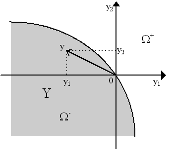
An example of a production set Y in two dimensional space is shown in Figure 1 where a particular production plan, the net production vector y = [y₁, y₂], is shown. Note that at that vector, y₁ is treated as an input (and hence takes a negative value) and y₂ as an output (and thus has positive value). Note how the axioms above imply that Y is something like that shown below (although an interesting alternative is where the boundaries are straight line, i.e. the case of constant returns to scale.).

Note that if we held drew Y for only two outputs holding all other outputs and all inputs constant, then we would effectively have the production possibilities frontier and the area below it so familiar from microeconomics principles. Similarly, if we drew Y for only two inputs and held all other inputs and all outputs constant, we would effectively have an isoquant and the area above it. All the analysis which follows, thus, has its analogues in the familiar Paretian isoquant and PPF worlds. Thus, this axiomatic, set-theoretic Y represents a generalization of these familiar concepts without assumptions about anything being held constant, or differentiability, etc. This generalization was the great advance provided by the activity analysis research at the Cowles Commission during the 1940s and 1950s

(2) Technical Efficiency

We now turn to technical aspects of production, specifically attempting to outline what is meant by technological efficiency in this activity analysis context. We define this as follows:

Technological Efficient Plan: a production plan y* Î Y is "technologically efficient" (t.e.) if there is no y Î Y such that y > y*.

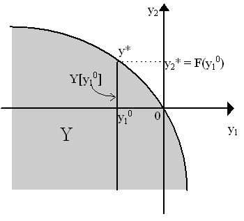
In Figure 1, the set of technologically efficient points is evidently the upper boundary of the production set Y. The particular y shown in the diagram, however, is not technologically efficient.

To prove the existence of technologically efficient points in the set Y, we need three lemmas and the working definition of a new concept, a subset of Y which we shall call Y[y_-i⁰] = {y Î Y ½ y_-i = y_-i⁰ }, i.e. we are definining the "set" Y[y_-i⁰] as a set of vectors in Y such that all elements in those vectors other than the ith element is fixed at some given level. Thus, the vector y_-i is defined as the vector with all elements but the ith and y_-i⁰ is the set of "fixed values" for these other elements. Thus only the ith element, y_i is free.

We can think of this set, Y[y_-i⁰] as a set within Y of one dimension less than Y. Figure 2 may help: here, all except y₂ is fixed - which, in a two-dimensional space, implies that y₁ is held fixed at y₁⁰ while y₂ fluctuates - so Y[y_-2⁰] = Y[y₁⁰] which is the thick line shown in Figure 2 (a subset of Y). Thus, a vector such as y* = [y₁⁰, y₂*] is an element of Y[y₁⁰] as well as Y.

Here are three lemmas we need regarding the production set with fixed factors:

Lemma 1: Y[y_-i⁰] is closed.

Proof: Suppose we take a convergent sequence {y^k} ® y*. As Y is closed, then y* Î Y. Let us suppose that y^k = [y_i^k, y_-i⁰], i.e. all vectors in the sequence have the same value for the elements other than i, i.e. only the ith varies in the sequence. Thus, the sequence {y^k} is a movement "along the line" Y[y_-i⁰] in Y. We know y* Î Y, but is y* Î Y[y_-i⁰] ? Actually, yes: as {y^k} ® y*, then y_iⁿ ® y_i* (ith element converges). As the other elements are fixed, then y* = [y_i*, y_-i⁰] which is an element of Y[y_-i⁰] by definition of this set. Thus, the set Y[y_-i⁰] is closed.§

Lemma 2: Y[y_-i⁰] is bounded, i.e. there is b Î Rⁿ such that y < b for all y Î Y[y_-i⁰].

Proof: Suppose not. Then then there is no such b Î Rⁿ. Or, for any m Î R, there is a y_i^m such that y_i^m > b and y^m = [y_i^m, y_-i⁰] Î Y[y_-i⁰]. We can presume y_i^m is an integer, thus 1/y_i^m Î [0, 1]. Let us then define divide the vector y^m by this integer: (1/y_i^m)y^m = [1, y_-i⁰/y_i^m]. This is a strange vector, but it is actually in Y. How do we know? Recall that Y is convex (Axiom 5) and that 0 Î Y (Axiom 1). Thus, as (1/y_i^m) Î [0, 1], then we can consider (1/y_i^m)y^m as the convex-combination between two points in Y: y^m and 0, i.e. (1/y_i^m)y^m = (1/y_i^m)y^m + (1- 1/y_i^m)0. By the convexity of Y, then (1/y_i^m)y^m Î Y. As we presumed that y_i^m > b for any number b, then we can take y_i^m to infinity. Doing so, then the vector (1/y_i^m)y^m = [1, y_-i⁰/y_i^m] ® [1, 0] as y_i^m ® ¥ . However, this vector [1, 0] Î Y is strictly in the positive orthant. By Axiom (2) on Y, we know this cannot be. Contradiction. Thus, Y[y_-i⁰] is bounded.§

Let us now define the efficiency function F[y_-i⁰] as:

F[y_-i⁰] = max y_i s.t. y Î Y[y_-i⁰].

Thus, F[y_-i⁰] is the set of greatest ith elements in vectors y of subset Y[y_-i⁰] (see Figure 2 for intuition). A "technologically efficient" vector y* can thus be defined as y* = [F[y_-i⁰], y_-i⁰] - or, equivalently, y* = argmax F[y_-i ⁰] (i.e. the arguments, y, that maximize the efficiency function, F[y_-i⁰]). Let us proceed to the next lemma:

Lemma 3: if Y is convex, then the efficiency function F[y_-i⁰] is concave.

Proof: Y is convex: take two vectors, y¹ and y² in Y and we know that l y¹ + (1-l )y² Î Y. Let us take two technologically efficient points, i.e. let y¹ = [F[y_-i¹], y_-i¹] and y² = [F[y_-i²], y_-i²]. By the convexity of Y, then:

l y¹ + (1-l )y² = [l F[y_-i¹] + (1-l )[F[y_-i²], l y_-i¹ + (1-l )y_-i²] Î Y

But by the definition of an efficiency function, F[l y_-i¹ + (1-l )y_-i²] ³ y_i " [y_i , l y_-i¹ + (1-l )y_-i²] - this includes y_i = l F[y_-i¹] + (1-l )[F[y_-i²]. Thus, it must be that F[l y_-i¹ + (1-l )y_-i²] ³ l F[y_-i¹] + (1-l )[F[y_-i²], thus the efficiency function is concave.§

We can now turn to the main theorem:

Theorem: (Existence) There exists a set of technologically efficient points in Y.

Proof: Recall that a "technologically efficient" vector y* is defined as y* = [F[y_-i⁰], y_-i⁰] or y* = argmax F[y_-i ⁰]. It is readily seen that F[y_-i⁰], which we know is concave, is also a continuous function. We already know from our first two lemmas that Y[y_-i⁰] is closed and bounded and thus compact. Therefore, by the Weierstrass Theorem, the efficiency function is continuously defined over a compact set and thus it attains an extremal in Y[y_-i⁰]. By concavity, y* = [F[y_-i⁰], y_-i⁰] is a maximum, thus there exists a set of technologically efficient points in Y.§

(3) The Producer's Decision

Let us now add some behavior to this and consider the issue of the profit-maximizing decision of the producer.  By definition:

Profit-Maximizing Plan: production plan y* is "profit-maximizing" for a given p if py* > py for all y Î Y.

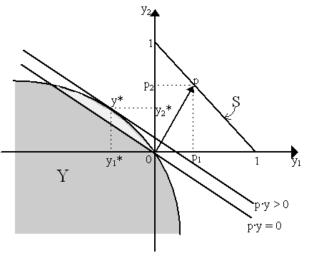
This is illustrated in Figure 3 where we have taken a particular price vector p = [p₁ p₂], some point in the unit simplex S Ì R², and the defined the price hyperplane p·y as a hyperplane orthogonal to vector p. Obviously, y* = [y₁*, y₂*] is the profit-maximizing point as p·y* > 0 The lightly-shaded area in Figure 3 is the set of feasible plans which yield positive profits at prices p.

We can define a "profit-function" as

p(p) = max py s.t. y Î Y

i.e. it is a mapping from prices (p Î Rⁿ) to some real number ("maximum profit"). (see here for the Paretian equivalent). The set of profit-maximizing points can be defined as:

P(p) = argmax p (p) = argmax  py s.t. y Î Y

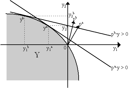
i.e. the arguments, y Î Y, that maximize profits.  Equivalently, P (p) = {y Î Y ½ py > py’ " y’ Î Y}. Thus, p (p) = pP (p). We can refer to P (p) as the "supply correspondence". An illustration of the principle follows for two prices in Figure 4.

In Figure 4, we have two sets of prices, p^a and p^b which. yield profit-maximizing activities y^a = Õ (p^a) and y^b = Õ (p^b). Now, we can tell that, in relative terms, p₂^a/p₁^a < p₂^b/p₂^b thus the price of the output (good 2) is higher at b. This implies that more of good 2 will be supplied at p^b than at p^a and more of good 1 will be demanded as input (i.e. y₁ is more negative at Õ (p^b)). Thus, the supply correspondence Õ (p) implies that as price of good 2 rises relative to good 1, more of good 2 will be produced, i.e. "supplied"; and more of good 1 will be demanded.

The following properties can be easily shown (see here for the Paretian equivalents)

Property 1: p(p) is homogeneous of degree 1 in prices.

Proof: p (p) = max py s.t. y Î Y. Let a ³ 0. Thus, p (a p) = max a py s.t. y Î Y = a [max py] s.t. y Î Y = a p (p). Thus, p (a p) = a p (p).§

Property 2: p(p) is a convex function.

Proof: Consider two prices, p¹, p² and two allocations y¹ , y² Î Y which are the equivalent profit-maximizing allocations, i.e. y¹ Î P (p¹) and y² Î P (p²). As Y is convex, then l y¹ + (1-l )y² Î Y. For ease of notation, define yl = l y¹ + (1-l )y². By the definition of profit-maximization, p¹y¹ ³ p¹yl , p²y² ³ p²yl . Thus multiplying the first by l Î (0, 1) and the second by (1-l ), then: , l p¹y¹ ³ l p¹yl + (1-l )p²y² ³ (1-l )p²y². Adding pointwise, we see immediately that: , l p¹y¹ + (1-l )p²y² ³ (l p¹ + (1-l )p²)yl . We can rewrite this in terms of profit functions as l p (p¹) + (1-l )p (p²) ³ p (l p¹ + (1-l )p²). Thus the profit function is convex.§

Property 3: (Law of Supply) "Supply of Output i" increases with price of that output, "Demand for Factor i" decreases with the price of that factor.

Proof: "Output supply" and "factor demand" are merely the profit-maximizing points, y Î P (p). Convexity of Y gave us convexity of the profit function (Property 2) and now we want to show that convexity of profit function yields an "upward-sloping" output supply curve and a "downward-sloping" factor demand curve. For simplicity, then, we shall assume twice differentiability of profit functions. Now, recall that p (p) = py. Thus, differentiating with respect to the ith element of the price vector, dp (p)/dp_i = y_i + å _i p_i(dy_i/dp_i). By the "envelope theorem", the term on the right collapses to zero so that we obtain the familiar "Shephard’s Lemma": dp (p)/dp_i = y_i where y_i is the ith element of y. Differentiating the profit function again, dp (p)/dp_i = dy_i/dp_i. Thus, by convexity of the profit function, dp (p)/dp_i ³ 0 and so dy_i/dp_i ³ 0. If y_i is positive (i.e. an output) this translates to "supply of output i" increases as p_i increases. If y_i is negative (i.e. a factor) this translates to "demand for factor i" decreases as the price of that factor increases.§

Property 4: p(p) is continuous and P(p) is upper semicontinouous.

Proof: p(p) = py s.t. y Î Y. By definition of inner products and linear functionals, py is jointly continuous in p and y; as Y is a "constant correspondence of p", it is both upper semicontinuous and lower semicontinuous. Applying Berge’s Theorem, then, p(p) is continuous and P(p) is upper semicontinuous.§

Theorem: There exists a set of profit maximizing points P (p).

Proof: p (p) is a continuous function (Property 4) defined over a closed set that is bounded above. A relatively weaker version of the Weierstrass Theorem implies that this function attains a maximum over Y. Thus, profit-maximizing points exist, i.e. P (p) exists.§

(4) The Efficiency of the Producer

It is apparent from Figure 3 that the profit-maximizing point y* is also a technically efficient point. Similarly, it is conceivable that all technically-efficient points can be achieved as profit-maximizing plans provided one finds the appropriate set of prices. The following two theorems state this clearly. Note that the phrase universality of markets" merely means that p >> 0.

Theorem: (p -max ® t.e.) If y* is profit-maximizing at p and there is universality of markets (p >> 0), then y* is technologically efficient.

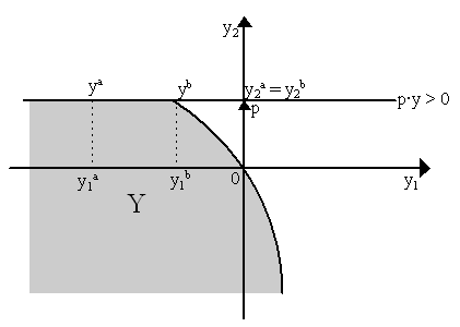
 Proof: Suppose not. Suppose y* is profit maximizing but it is not t.e. Then by definition there is a y Î Y such that y > y*. Premultiplying by p (recall, p >> 0), then py > py*. Thus y* could not have been profit-maximizing. Contradiction.§

Figure 5 illustrates why the assumption of universality of markets is required. At the given p shown in Figure 5 (where p₁ = 0) there are several production vectors y which are profit maximizing (e.g. y^a and y^b), yet note that y^b is technically efficient whereas y^a is not because y^b > y^a (i.e. y^b = [y₁^b, y₂^b] > [y₁^a, y₂^a] = y^a). Thus, y^a is a profit-maximizing point but it is not technologically efficient

We now turn to the converse theorem:

Theorem: (t.e. ® p -max) If y* is technologically-efficient, then there is a p (¹ 0) such that at this p, y* is profit-maximizing.

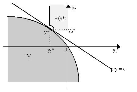
 Proof: For this, we need the Separating Hyperplane Theorem (SHT). Define two sets: Y (the regular production set) and the following H(y*) = {y Î Rⁿ ½ y >> y*} which we wish to separate (cf. Figure 6 for heuristics). They both need to be non-empty, convex and disjoint. For Y, this is easy: by assumption (1), 0 Î Y, thus it is non-empty. Similarly, by assumption (5), Y is convex. Finally, by the definition of H(y*) and "technological efficiency" of y*, Y has no points in common with H(y*).

H(y*) is also non-empty: i.e. take a vector e > 0. Then y* + e >> y*. Thus, y*+e Î H(y*). Thus, H(y*) is non-empty. H(y*) is also convex: take two vectors, y¹ and y² in H(y*). Thus, y¹ >> y* and y² >> y* by definition. Let take l Î (0, 1) and premultiply the inequalities by l and (1-l ) respectively so that l y¹ >> l y* and (1-l )y² >> (1-l )y*. Add these two together pointwise: l y¹ + (1-l )y² >> l y* + (1-l )y* = y*. Thus, the convex combination of y¹ and y² is strictly greater than y*. Thus, l y¹ + (1-l )y² Î H(y*), thus H(y*) is convex.

Hence, we have two non-empty, convex and disjoint sets H(y*) and Y. Apply SHT. There is a pair (p, c) where p Î Rⁿ and p (¹ 0) and c Î R such that:

py £ c " y Î Y

py ³ c " y Î H(y*)

Now, let us define a positive vector e > 0 and a number n > 0 so we can define the vector [y* + (1/n)e ]. Thus, by definition, [y* + (1/n)e ] >> y* and thus, by definition, [y* + (1/n)e ] Î H(y*). From the SHT, then, we know that p[y* + (1/n)e ] ³ c ³ py " y Î Y. Taking n ® ¥ , then we see that py* ³ py " y Î Y. This is the definition of y* as a profit-maximizing point.§

A diagrammatic illustration (slightly exaggerated for effect) of the theorem can be conceived in Figure 6.

The meaning of these equivalence theorems is not entirely vacuous - particularly in light of the Socialist Calculation debate. It implies, quite simply, that any technically efficient outcome can be achieved in a "capitalist" economies by profit-maximizing behavior - as long as "one gets the prices right". Conversely, it also implies that centrally-planned economies can achieve technically efficient outcomes - provided the planning board "gets the prices right" and requires that the managers of state enterprises maximize profit/minimize cost. These equivalence theorems were central to Abba Lerner (1934) and Oskar Lange (1936), although they expressed them in Paretian context. The Neo-Walrasian version here, due to Tjalling Koopmans (1951), thus lent support to the Lange-Lerner contention.

(5) Marginalism

Let us connect the production idea back to the Paretian notion of differentiable "marginalism" - more specifically, the idea that output/inputs will be chosen by producers where the marginal rates of technical substitution (MRTS) are equal to price ratios. Let us assume universality of markets so that p >> 0. Consider y Î P (p). By our second equivalence theorem outlined above, y Î P (p) Þ y = [F[y_-i⁰], y_-i⁰], i.e. y is a technically efficient point. Let us consider another technologically efficient point [y + e e_j] = [F[y_-i⁰ + e e_j], y_-i⁰ + e e_j] where e ¹ 0 and j ¹ i. By definition of profit maximization, then, py ³ p[y + e e_j], or:

p_iF[y_-i⁰] + p_-iy_-i⁰ ³ p_iF[y_-i⁰ + e e_j] + p_-i[y_-i⁰ + e e_j]

where p_i is the price of the ith good and p_-i is the vector of price of all goods except i. Rearranging:

p_i [F[y_-i⁰] + F[y_-i⁰ + e e_j] ³ p_-i[y_-i⁰ - y_-i⁰ + e e_j] = e p_j

Thus, dividing by p_i:

[F[y_-i⁰] + F[y_-i⁰ + e e_j] ³ e p_j/p_i

We now wish to divide by e but we have not placed any restrictions on e except that it be non-zero. Thus, if e > 0, this becomes:

[F[y_-i⁰] + F[y_-i⁰ + e e_j]/e ³ p_j/p_i

or

[F[y_-i⁰ + e e_j] + F[y_-i⁰]]/e £ - p_j/p_i

whereas if e < 0, then:

[F[y_-i⁰] + F[y_-i⁰ + e e_j]/e £ p_j/p_i

or

[F[y_-i⁰ + e e_j] + F[y_-i⁰]]/e ³ - p_j/p_i

Thus, taking the limit, as e ® 0, we obtain:

[dF/dy_j]⁺ £ -p_j/p_i

and

[dF/dy_j]^- ³ -p_j/p_i

But dF/dy_j is merely dy_i/dy_j. Thus, this implies that if "differentiable", then:

- dy_i/dy_j = -[dF/dy_j] = p_j/p_i

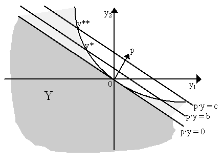
or, simply, the very familiar claim that the marginal rate of technical substitution (MRTS) between goods i and j (i.e. - dy_i/dy_j) is equal to the reciprocal ratio of their prices.

(6) Competition

We have so far kept the assumption that Y is convex and thus maintained non-increasing returns. Naturally, if the production set Y is non-convex so as to allow for "increasing returns to scale" or if we also disallowed decreasing returns, then what would happen?

Increasing returns is implied if the production set is non-convex. This would remove the concavity of the efficiency function but it would not implicate the first equivalence theorem (profit-maximizing points remain technically efficient). However, it would affect the existence of profit-maximizing points (or rather, those points and associated profits would be either infinite or non-positive) and thus the second equivalence theorem would be completely disabled. This is quite easy to visualize, as in Figure 7 where we have a non-convex Y (i.e. Y with increasing returns to scale). We see that the lightly shaded area represents the area of Y which yields positive profits (i.e. where p·y > 0 for a given p). Note that y* is not profit maximizing at the given price p as y** yields even greater profits, i.e. py* = b < c = py**. Thus, we can conceive that in this situation, at a given p, there are no profit-maximizing points in Y and no limit to the amount of output produced (or rather, the firm will produce until monopoly).

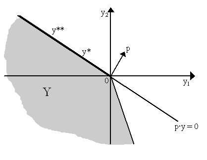
Note that as "increasing returns" are required for any discussion of monopolistic or imperfect competition, then the assumption of convexity of Y implies that we must rule imperfectly competitive situations out. What if there is only a small portion of the production set that is non-convex? We might conceivably, in that case, still be able to define profit-maximizing points, but the associated supply correspondence would be discontinuous. This might be problematic for existence of equilibrium if the demand function passes through that hole in the supply function. However, as conjectured by M.J. Farrell (1959) and Jerome Rothenberg (1960) and proved by Ross M.  Starr (1969), one can tolerate some amount of non-convexity as the process of aggregation will tend to "convexify" the aggregate production set and thus fill in the holes in the aggregate supply correspondence. For more reflections on incorporating non-convexities and imperfect competition in general equilibrium theory, see Negishi (1961), Arrow (1971) and Arrow and Hahn (1971: Ch.6, 7) and attempts using non-smooth differentials are surveyed in Quinzii (1992) and Brown (1991) and in our discussion of non-convexity.

However, is convexity equivalent to perfect competition? Not quite. The possible existince of diminishing returns to scale not only is logically troublesome, but the existence of positive profits may itself imply that entry is not exactly "free". Many G.E. theorists have tried to make arguments for the retention of diminishing returns on the basis of goods "private" to the firm or by choosing a private-ownership economy and thus reallocating that profit to agents. However, others have chosen to replace the simple convexity assumption outright and assume instead that production is a "convex cone", i.e. for any y¹, y² Î Y and any a ³ 0, b ³ 0, it is true that a y¹ + b y² Î Y. This, in turn, implies "constant returns" as it rules out both increasing and decreasing returns to scale. This is shown heuristically in Figure 8.  

The assumption of constant returns or that Y is a "convex cone" essentially implies that the "bounds" of the production set are straight and thus the profit-maximizing points are either indeterminate (along the boundary of Y, y* and y** are equally profitable at p) or zero (no production at all). In our diagram, this implies that there is a unique price that can yield a positive profit-maximizing output yet, at that price, the profit-maximizing plan is actually indeterminate. As is obvious from Figure 8, any other p would imply that profit-maximizing output is the origin, 0 Î Y, and thus inactivity. For an analogue, recall that constant returns to scale implies that, in a supply-and-demand diagram, the supply curve is horizontal, thus there is a unique p where output is supplied but at this p, the actual output is actually indeterminate (or rather, in equilibrium, it is determined by the demand function and thus the consumer decision). Note also that a convex cone production set necessarily implies zero profits, thus fitting better with Walras's "perfect competition" idea of "no gains, no losses" to the entrepreneur.

We should note that the assumptions of divisibility (if y Î Y, then l y Î Y where l Î [0, 1]) and additivity (if y¹, y² Î Y, then y¹ + y² Î Y) of activities in Y are enough to give us a convex cone.

Theorem: If production is divisible and additive, then Y is a convex cone.

Proof: Y is a "convex cone" if for any y¹, y² Î Y and any a ³ 0, b ³ 0, it is true that a y¹ + b y² Î Y. Divisibility implies that ly¹ Î Y and (1-l )y² Î Y for l Î (0, 1). By additivity, l y¹ + (1-l )y² Î Y, which implies convexity. Consider now any particular a ³ 0. Let n be the largest integer not exceeding a , then l = a - n Î (0, 1). By divisibility, then, if y Î Y, then l y = (a - n)y Î Y. Consider the set of vectors {yⁱ}ⁿ_i=1 where yⁱ = y. Thus, by additivity, å _i=1ⁿ yⁱ = ny Î Y. Let yⁿ⁺¹ = l y, then by additivity å _i=1ⁿ⁺¹ yⁱ = ny + l y = a y. As ny Î Y and l y Î Y, then by additivity a y Î Y. This was true for any a ³ 0. Thus, Y is a convex cone.§

(7) Aggregation

Let us now reintroduce our firm index, f . Thus we can define for each firm f Î F, a profit function and a supply correspondence:

p ^f (p) = max py s.t. y Î Y^f

P ^f(p) = argmax py s.t. Y Î Y^f

Thus the supply correspondence is P ^f(p) = {y Î Y^f ½ py > py’ " y’ Î Y^f}.

Now, let us define the "aggregate production set" as Y = å _fY^f. We can also define a profit function and supply correspondence for the aggregate as:

p (p) = max py s.t. y Î Y

P (p) = argmax py s.t. Y Î Y

Now, we would like to know whether "aggregate supply", defined as the result of profit maximization over the "aggregate" production set, can also be found by summing up the individual supplies from individual firm profit-maximization. To show this, we first need a lemma - that the profit functions are equal:

Lemma: p (p) = å _f p ^f(p)

Proof: Step (i): By definition of the aggregate production set, å _f y^f Î Y. By definition of profit-maximization, p (p) ³ py " y Î Y. Thus, p (p) ³ p(å _f y^f) " y^f Î Y^f. Thus, p (p) ³ å _f py^f " y^f Î Y^f. Thus, p (p) ³ å _f p ^f(p).

We can now turn to the main theorem on the equivalence of the supply corresponence over the aggregate set and the sum of individual supply correspondences over individual sets:

Theorem: P (p) = å _f P ^f(p)

Thus the aggregate supply correspondence is the same as the sum of the individual supply correspondences.

Selected References

Kenneth J. Arrow (1971) "The Firm in General Equilibrium Theory", in R. Marris and A. Wood, editors, The Corporate Economy: Growth, competition and innovative potential. Cambridge, Mass: Harvard University Press.

Gerard Debreu (1959) Theory of Value: An axiomatic analysis of economic equilibrium. New York: Wiley.

David Gale. (1960) The Theory of Linear Economic Models. New York: McGraw-Hill.

Tjalling C. Koopmans (1951) "Analysis of Production as an Efficient Combination of Activities", in Koopmans, editor, Activity Analysis of Production and Allocation: Proceedings of a conference. New York: Wiley.

Tjalling C. Koopmans (1957) Three Essays on the State of Economic Science. New York: McGraw-Hill.