|
Contents (A) The Walrasian Exchange Economy (A) The Walrasian Exchange Economy "Walrasian" pure exchange refers to the price-mediated process of exchange of endowments of goods (i.e. no production) as initially outlined by William Stanley Jevons (1871), Léon Walras (1874), Irving Fisher (1892), Vilfredo Pareto (1896, 1906) and others. The basic story is simple and can be outlined as follows:
In its most general form, a pure exchange Walrasian equilibrium can be defined abstractly as follows. Let there be H households and n goods. Each household is characterized by preferences (denoted ³ h for the hth household) and an endowment vector (denoted eh for the hth household). We can often represent preferences by a "utility function", which we denote uh for the hth household. As eh , the endowment of household h, is a vector, then we can define the hth household's individual endowment of the ith good as eih. As we have H households, then we can define the economy-wide or aggregate endowment of the ith good as the sum of all the household's individual endowment of the ith good, i.e.:
Each household takes the prices of goods, which we denote by the vector p, as given and attempts to choose a consumption bundle (a vector denoted xh for the hth household) which maximizes their utility. We place the restriction that the bundle xh chosen by the hth household is affordable to that household, thus its value pxh cannot exceed the value of the household's budget (peh). Thus, the utility-maximizing program of the household is:
From the solution to this program, we can define the desired bundle xh. As xh is a vector, then the ith entry of that vector, call it xih, reflects household h's individual demand for the ith good. The difference between household h's individual demand for good i and its individual endowment of good i is often referred to as the household's net demand. If net demand for good i is positive (i.e. the household demands more of good i than it has), then we shall denoted it as D ih; it net demand for good i is negative (i.e. the household demands less of good i than it already has), then we denote its absolute value by Oih. Thus, D ih reflects the amount of good i household wishes to obtain from the market, while Oih reflects the amount of good i that the household is offering to the market. Thus, D ih, Oih for a variety of goods i = 1, .., n, express the household's desired trades. As we have a total of H households, then the market demand for the ith good is merely the sum of each household's individual demand for the ith good, i.e.
is the market demand for the ith good. A Walrasian pure exchange equilibrium is then defined as a price vector (p*) and a set of consumption bundles (xh*, one for each household), with the following properties:
The second part of the definition is the familiar one that the "demand" for a good must be equal to the "supply" of a good in equilibrium. Notice that after some algebraic substitution, we can write Condition (2) as:
Thus the desired trades, on the whole, must be met. Notice that the first part of the definition of Walrasian equilibrium argues that it must be established according to price-mediated exchange process: i.e. households take prices as given and express their desired trades with "the market" and not "with other agents". An equilibrium is thus associated with a price vector, p*, that leads agents to make net demands and offers such that the markets "clear". We leave the rest of the analysis of Walrasian pure exchange equilibrium in abstract form to our more detailed discussion of Walrasian general equilibrium theory. What we shall do here is merely review several diagrammatic representations of Walrasian pure exchange. We begin with the "demand-and-supply" apparatus developed by Philip H. Wicksteed (1910, 1914), from which we will then derive the excess demand function representation. We then represent Walrasian pure exchange via the "Edgeworth-Bowley box" introduced by Pareto (1906), and consequently derive a representation of equilibrium via price-consumption curves and, finally, net trade diagrams. All of these diagrams are legitimate representations of the same thing - Walrasian pure exchange (albeit at a low level of dimensionality) -- and all are extremely useful. There are advantages and disadvantages to each diagram, as they emphasize different aspects of Walrasian exchange, but it is important to note that, at least in principle, the same story goes on in each. (B) Demand-and-Supply Representation The determination of equilibrium in a market boils down to constructing a "demand-and-supply" structure. However, as we are dealing with pure exchange, thus Marshallian "supply" curves are not available, as these are derived from production. How do we obtain the demand-and-supply apparatus in pure exchange? The following presentation is due largely to Philip H. Wicksteed (1910, 1914). As we are in a price-mediated process, agents take prices as given. Let us have two goods, x1 and x2. Consider household h. We denote by eh = (e1h, e2h) the hth household's endowment of the two goods and his utility function by uh. The objective of the hth household is to maximize utility subject to a given price constraint:
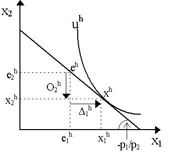
thus the left side of the budget constraint refers to the hth consumer's expenditures on goods and the right side of the constraint refers to revenue received from the sale of his endowments. Note that we do not subsume the endowment here under the banner of "income". The consumer's decision is depicted in Figure 1. The slope of the budget constraint is -p1/p2, the ratio of the market price of good 1 to the price of good 2. These are "given" to him.
In Figure 1 we have two points indicated on the budget line: the tangency point xh = (x1h, x2h), where our individual would like to consume, and the endowment point eh = (e1h, e2h). These points, as is obvious, do not coincide: our consumer possesses more than he desires of good x2 and less than he desires of good x1. It is in his interest, therefore, to increase his consumption of x1 by D1h but his budget does not allow it. In order to increase consumption of the first good by D1h, he must sell some of his endowment of the second good (portion O2h in Figure 1) to the "market" and use the revenue of that sale to make his desired purchases. As is obvious:
D1 and O2 are, in effect, the consumer's "net demand" for good x1 and "offer" of good x2, respectively. As he uses the revenue of the sale to make his purchases, then it is necessary that:
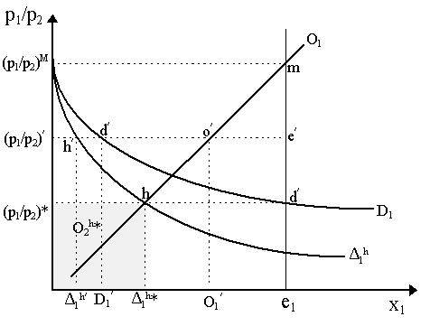
the value of the purchase be equal to the value of the sale. The consumer's total demand for the first good is x1h = e1h + D1h, whereas his total demand for the second good is x2h = e2h - O2h. At different price ratios p1/p2, the hth household may be willing to demand/offer less or more of each good than this. By figuring out what the hth household would demand/offer at different price ratios, we can construct the demand and offer curves of the individual. In Figure 2, we have constructed the net demand curve for agent h, D 1h. As we see, it is a negative function of the price ratio, p1/p2: the greater the price of good 1 relative to good 2, the less he is willing to purchase of good 1. At prices, (p1/p2)*, he demands D1h* from the market, shown by point h in Figure 2. Notice that rearranging our purchase-sale equality, we see that:
Thus, the hth consumer's corresponding offer of good x2, O2h*, is the shaded rectangle in Figure 2 below the.
The shape of the individual h's demand curve D 1h seems to make sense, but let us consider them a bit more carefully. If the price ratio p1/p2 rises, what happens to the quantities demanded of good x1 and offered of good x2? Holding everything else constant, when the price ratio rises, we would now have p1D 1h > p2O2h, thus the consumer is offering too little of good x2 for the amount of good x1 he desires to obtain. There are effectively two things he can do to bring his expenditure-sale relationship back into equality: he can increase the amount offered O2h, or he can decrease his demand for the first good D 1h. Chances are he will do a little bit of both. Thus, in Figure 1, we see that when prices rise from (p1/p2)* to (p1/p2)¢ , his demand for good x1 declines from D 1h* to D 1h¢ (from point h to point h¢ in Figure 2). What about his offer of the second good? In principle, as we noted, because it is now costlier to exchange x2 for x1, he will probably increase the amount offered of good x2 if he does not want to be forced to reduce D 1h too much. In this case, the area of the rectangle under h¢ would be greater than the area under h (i.e. O2h increases). However, getting rid of good x2 implies a loss in utility. Thus, not only is he getting less utility from buying a smaller amount of x1, he is losing even more utility because he has to get rid of something he rather likes, good x2. His preferences may thus be such that when p1/p2 rises, he thinks it worthwhile to decrease both the amount offered of good x2 and the amount desired of good x1. In this case, O2h falls, so that the area of the rectangle under h¢ is smaller than the rectangle under h. In sum, we can think of the first case, when offer O2h increases with a rise in p1/p2, as reflecting a situation where x1 matters a lot to him and x2 matters relatively little; the second case, when offer decreases with a rise in p1/p2, reflects the reverse reasoning. However, there is another side of the coin to this story. As p1 rises relative to the p2, this implicitly means that p2 is falling relative to p1. Thus, we can plot agent h's offer of x2 as a function of p2/p1. Now, the story we have just told says that the offer of x2 can either rise or fall when p2/p1 falls: in the first case, O2h rises in response to a fall in p2/p1; in the second case, O2h fall in response to a fall in p2/p1. Thus, agent h's offer curve can be downward or upward sloping with respect to its relative price, p2/p1. Perhaps it can even be both: upward sloping at some prices, downward sloping at others. This ambiguity is not as paradoxical as it sounds. As John Hicks (1939:p.36-37) reminds us, this is particularly apparent in labor-leisure choice: as wages increase, a worker may gain an incentive to work more and thus acquire more money to consume even more goods; at the same time, this means he gets more money for less work and thus may value his leisure enough to reduce his working hours. The familiar "backward-bending" labor supply curve we find in labor economics reflects this reasonable "paradox". But let us not spend too much time fretting over this: the only important thing to keep in mind at this point is that agent h's offer curve O2h can be derived entirely from his demand curve D1h. Let us now turn to equilibrium. Remember that D 1h is household h's net demand for good x1 from the market, while O2h is his offer of good x2 "the market". There are other people in the market as well who may themselves offer and demand goods x1 and x2. They are also endowed with goods x1 and x2. Let us focus entirely on good x1 for the moment. Let there be H consumers. Then, the total endowment of good x1 in the economy is:
where e1k is the kth consumer's endowment of good 1. Total economy-wide endowment is fixed. This is denoted in Figure 2 by the vertical line e1. Suppose, for the moment, that only consumer h is demanding good x1 from the market. All the others are either consuming their own endowment of good x1 (i.e. withholding it from the market) or offering it for sale. Thus, let O1 denote the market offer of good x1 by all consumers other than h, i.e.
where O1k is the offer of good x1 by agent k. Now, as we know, consumers will only offer something on sale to the market if they are demanding something else from the market. In this case, as we only have two goods, the offers of good x1 by the other agents implies they are making net demands for good x2. Suppose for the moment, that the other agents have an "upward sloping" offer curve: so, when p1/p2 rises, they offer more of good x1 for sale. This is captured in Figure 2 by the upward-slope of the curve O1. This is the "supply curve" that consumer h faces in the market for good x1. Notice the important fact that, as we have shown in our previous analysis, the offer curve of one good is derived from the net demand of the other good. There is no production in this model: the upward sloping offer or "supply" curve of x1 is derived solely from net demand for good x2. Thus, as Wicksteed notes famously writes:
To see this, let us now derive Wicksteed's total demand curve D1 in Figure 2 which adds up the desired consumption of good x1, i.e. D1 = å k=1H x1k, where x1k is the agent k's desired consumption of good x1k. Now, we stipulated that only agent h was making net demands of good x1 on the market, and all others were offering good x1. However, this does not mean that they are not consuming x1: recall that O1k = e1k - x1k, their offer to the market of good x1 is merely the portion of their individual endowments that they do not wish to consume themselves. The shape of the total demand curve D1 can be deciphered easily. Suppose prices are (p1/p2)¢ , so agent h's net demand is D 1h¢ while all the other agents together offer O1¢ , as shown by their offer curve. Now, examine the difference between O1¢ and the aggregate endowment e1 (i.e. the horizontal distance between points o¢ and e¢ in Figure 2). This difference, e1 - O1¢ , is nothing other than the amount of total endowment that is not offered on the market. Wicksteed refers to this as the reservation demand for good x1, i.e. agents' demand for their own endowment of good x1. Thus, the offer curve O1 reflects the idea that the lower the price p1/p2, the more agents will withhold good x1 from the market for self-consumption (and, of course, the more agent h will demand good D 1h from the market). Total demand D1 is net demand plus reservation demand, so the more agents demand of good x1 in terms of reservation, the greater will be the amount of total demand. The horizontal difference between O1 and e will be identical to the horizontal difference between D1 and D 1h. Similarly, the horizontal difference between O1 and D1h is identical to the horizontal difference between D1 and e1 (this is not apparent in this poorly-drawn diagram, but in Figure 2, the difference between h¢ and d¢ is supposed to be the same as the difference between o¢ and e¢ ; similarly, the difference between h¢ and o¢ is also supposed to be the same as the difference between d¢ and e¢ ). A market equilibrium is defined as when the offers of a good in the market are equal to the net demands for that good. In our case, D1h = O1. Will it also necessarily be that the total demand (reservation demand plus net demand) be equal to the endowment? Indeed this is so and verifying it is a matter of simple algebra. The difference between total endowments and the offers by agents other than h is:
As, by definition, O1k = e1k - x1k, then:
or simply:
but as e1h = x1h - D 1h:
Finally, by definition, D1 = å k=1H x1k, then:
Thus, the difference between the total endowment of good x1 (e1) and the amount all agents other than h offer (O1) is equal to the difference between the total demand for good x1 and the net demand by agent h of good. Equivalently, we could write this as:
so that the difference between net demand by agent h and offers by other agents (the "market difference") is identical to the difference between total demand and endowment. Thus, markets clear when O1 = D 1h or, equivalently, when D1 = e1. This is shown in Figure 2: at prices (p1/p2)*, the "market" of net demands and offers clears at point h while the "market" of total demands and endowments clears at point d. If we consider a higher price, say (p1/p2)¢ , where net demand by agent h is D 1h¢ ¢ while offers by all other agents are O1¢ , then as D 1h¢ < O1¢ , by the formula, we obtain the necessary result that D1¢ < e1¢ , as is obvious in Figure 2. Finally, notice that when the price ratio is (p1/p2)M, so that the entire endowment of good x1 is offered on the market, then necessarily D1 = D 1h = 0. Thus, as Wicksteed notes:
Finally, we should note the equivalent relationships in the converse market for good 2. As the offers of O1 by all agents but the hth are balanced by net demands for good 2, then we can define D 2 = å k=1H-1 D 2k as the net demand for good x2 by all "other" agents. Offers of good x2 are simply O2h. If we were to draw a similar diagram, we would note that:
where D2 = å k=1H x2k is total demand for good 2 and e2 is total endowment of good 2. As each agent is forced by his budget constraint to make expenditures equal to sale values, then p1D 1h = p2O2h for agent h and p1O1 = p2D 2 for the aggregate of all other agents. Putting these together:
which writtein in full yields:
or simply:
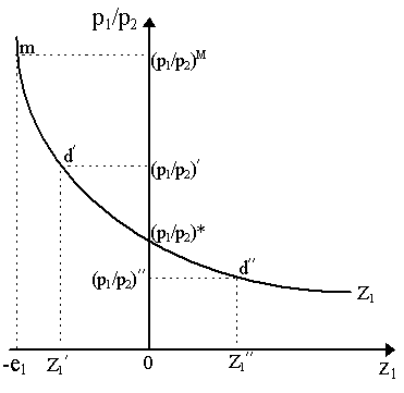
which is merely Walras's Law. Thus, if there is equilibrium in the market for good x1 (i.e. D1 = e1 or equivalently, D 1h = O1), then necessarily we obtain equilibrium in the market for good x2 (i.e. D2 = e2 or equivalently, D 2 = O2h). Finally, it might be worth mentioning that one can obtain an excess demand representation from the Wicksteedian demand-and-supply structure. Specifically, we can define Z1 = D1 - e1 as the market excess demand of good x1. This is shown in Figure 3 below. Notice that the excess demand function is merely the regular market demand D1 function we had in Figure 2 with the vartical axis transferred to the endowment line, e1. Otherwise, the Figure 2 and Figure 3 correspond to each other. For instance, at the equilibrium price, (p1/p2)* excess demand is zero, Z1 = 0, implying D1 = e1 as we had at point d in Figure 2. Similarly, when price rises to (p1/p2)¢ , excess demand falls to Z1¢ = D1¢ - e1 < 0 which corresponds in Figure 2 to point d¢ . If price falls to (p1/p2)¢ ¢ , excess demand is positive, Z1¢ ¢ > 0 (as also implied in Figure 2). Note that when price was at its "maximum", (p1/p2)M, in Figure 2, we said that D1 = 0, which implies in turn that the corresponding Z1 is merely -e1, as shown in Figure 3.
In sum, we see that the market excess demand function for good x1 depicted in Figure 3 contains effectively most of the information we had in Figure 2. The only difference is that we cannot differentiate between net demand/offers and total demand in Figure 3. However, it is worthwhile noticing one thing: as we know, in Figure 2, the difference between D1 and e1 is identical to the difference between D 1h and O1. Thus, we could define Z1 = D 1h - O1 without losing a beat, so that excess demands/supplies depicted in Figure 3 could be interpreted as the difference between net market demands and offers of good x1. (C) Edgeworth-Bowley Box Representation Walrasian pure exchange equilibrium can also be represented in the famous "Edgeworth-Bowley" box. This diagrammatic representation is originally due to Vilfredo Pareto (1906: p. 138), but the misleading name "Edgeworth-Bowley" has unfortunately become stuck among economists. The principle is the same as before, albeit for diagrammatic exposition must limit ourselves to two (at best two types) of agents, whom we shall call A and B, and two goods, x1 and x2. Let eA = (e1A, e2A) denote A's endowment of the two goods, and eB = (e1B, e2B) is the B's endowment of the two goods, thus total economy-wide endowment of good x1 is e1 = e1A + e1B and economy-wide endowment of good x2 is e2 = e2A + e2B. Once again, we must remember that Walrasian exchange is a price-mediated process, thus agents take the prices of the goods, x1 and x2 as given. In other words, they do not "see" each other or trade with each other directly; rather, they trade with "the market". Thus, each agent makes his demands and offers according to his utility-maximizing choice subject to a budget constraint. Agents face the same set of prices, p1, p2, so A's utility-maximizing program is:
while B's utility-maximizing program is:
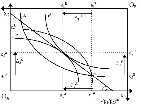
where xA = (x1A, x2A) is A's desired bundle and xB = (x1B, x2B) is B's desired bundle. Each one of these utility-maximizing programs can be represented in (x1, x2) space, where the desired bundle by an agent is the maximium indifference curve for that given budget constraint, as we had earlier shown for agent h in Figure 1. We can represent both the utility-maximizing programs of A and B in one diagram - the Edgeworth-Bowley Box in Figure 4 - by rotating B's version of Figure 1 and superimposing it on A's version of Figure 1. The "box" is formed by the corresponding axes. Thus, OA in the bottom left of Figure 4 represents the origin of agent A's picture, while OB in the top right is the origin of agent B's picture. The more we move to the northwest away from OA, we see A's indifference curves ascend, thus the greater the utility of agent A. In contrast, the more we moe to the southeast away from OB, we see B's indifference curves ascend, and thus the greater the utility of agent B.
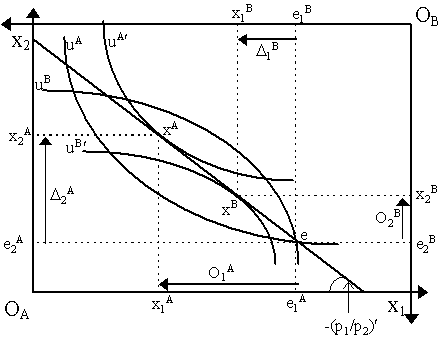
Figure 4 happens to show a Walrasian equilibrium. What this means is the following. Consider the endowment allocation, e, where agent A gets utility level uA and agent B has utility uB. Given the price ratio (p1/p2)*, we can form a budget constraint for each of the agents (they share the same budget line, as is obvious). Agent A's utility-maximization exercise leads him to the tangency of his highest indifference curve and the budget line, which happens to be point x in Figure 4, where he chooses bundle (x1A, x2A) and gains utility uA¢ . Consequently, in moving from the endowment point e to point x, he makes a net demand D 2A of good x2 from the market, and, in exchange, offers amount O1A of good x1 to the market. Conversely, consider agent B. Facing the same price, his utility at his endowment is uB. His utility-maximizing exercise also takes him to point x in Figure 4. At this point, his chosen bundle is (x1B, x2B) (the amounts are now read from the opposite origin, OB). Consequently, he has a net demand D 1B of good x1 and makes an offer of O2B of good x2 to the market. As it happens, as we see in Figure 4, the amount demanded of good x1 by agent B is equal to the amount offered by agent A, i.e. D 1B = O1A; conversely, the amount offered of good x2 by agent B is equal to the amount demanded by agent A, i.e. O2B = D 2A. Thus, both the market for good x1 and the market for good x2 will clear at prices (p1/p2)*. Thus, Figure 4 represents a Walrasian equilibrium. How does one depict a disequilibrium in an Edgeworth-Bowley box? As the Walrasian exchange process is price-mediated, a disequilibrium is defined as a "wrong price", i.e. a price where utility-maximizing agents will not make the corresponding net demands and offers of goods to the market such that the markets clear. This is shown in Figure 5, where we have price ratio (p1/p2)¢ . At this price, when agent A maximizes utility, he achieves bundle xA, while agent B achieves bundle xB. Both are points on the same price line, but they are not the same points. This implies that A's offer of good x1 is greater than agent B's net demand for that good, i.e. O1A > D 1B, while agent A's net demand for good x2 exceeds agent B's offer, i.e. D 2A > O2B. Thus, the markets for x1 and x2 do not clear. Thus, the situation in Figure 5 is a Walrasian disequilibrium.
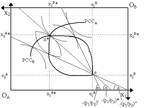
An easy way to trace out excess demands from the Edgeworth-Bowley box is via price-consumption curves (PCCs). To see these, examine Figure 6. Here we have depicted three prices, (p1/p2)¢ > (p1/p2)* > (p1/p2)¢ ¢ . At each price, we see the corresponding utility-maximizing points for agents A and B as represented by the tangency of their respective indifference curves and the corresponding budget constraint. Notice that at the highest price ratio depicted, (p1/p2)¢ , the indifference curves of agents A and B are both tangent to the corresponding price line, but they are not tangent at the same point. This means that, as we can decipher in Figure 6, at prices (p1/p2)¢ , agent A's offer of good x1 exceeds agent B's net demand for it, while agent B's offer of good x2 is not enough to satisfy agent A's net demand for it. Thus, the relativiely high price ratio (p1/p2)¢ implies there is an excess supply of good x1 and an excess demand for good x2 (as intuition would lead us to expect: when p1 is relatively high, much of x1 is offered and little demanded, while, at the same time, the relatively low p2 implies that much is demanded of x2 while little is offered). We do not have an equilibrium. In contrast, consider the the much lower price ratio, (p1/p2)¢ ¢ where, again, agent A and B's indifference curves are tangent to the relevant budget line, but not at the same point. As we see in Figure 6, agent A's offer of good x1 is not enough to meet agent B's net demand for it, while agent B's offer of good x2 exceeds agent A's net demand for it. In short, at the relatively low price ratio, (p1/p2)¢ ¢ , there is excess demand for good x1 while there is excess supply of good x2. Once again, we are not at equilibrium. Finally, notice that at (p1/p2)*, agents are tangent to the price line at the same point, implying net demands and offers for each good are equal, so we have equilibrium.
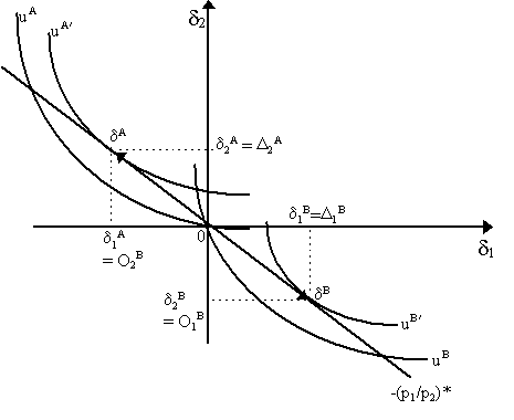
The thick black lines in Figure 6, PCCA and PCCB, denote the price-consumption curves of agents A and B resplectively. Effectively, PCCA traces out the utility-maximizing choices of agent A as prices vary, while PCCB traces the utility-maximizing choices of agent B as prices vary. Now, as we have already shown, a Walrasian equilibrium is achieved when the utility-maximizing choices of both agents at a given price lands on the same point. This will be precisely where the PCC curves intersect each other -- in this case, as we see in Figure 6, at point x*. The slope of a price line that passes through point x* and the endowment e is precisely the equilibrium prices, (p1/p2)*. The final diagrammatic representation of Walrasian pure exchange we shall consider is the net trade diagram. This is derived from a simple Edgeworth-Bowley box, and is particularly useful when trying to analyze economies with more than two agents for which the Edgeworth-Bowley box usually does not work. For the two-agent case, the construction process is simple. Consider our earlier Edgeworth-Bowley box in Figure 4, where we have two agents and two goods, etc. The equivalent net trade diagram is shown in Figure 7. To see how the derivation is, examine indifference curve uA¢ . Notice that it passes through the origin 0 in Figure 7 precisely where it passes through the endowment point e in Figure 4. Thus, it is as if we have placed the origin right on point e. Now, to obtain indifference curve uB¢ in Figure 7, go back to Figure 4 and swing the corresponding curve uB¢ by 45° on the endowment point. This should yield the result in Figure 7.
The price line passing through the origin in Figure 7 is precisely the same price line that passes through e in Figure 4, with slope -(p1/p2)*. Thus, maximizing utility, agent A goes to uA (at the tangency point d A) while agent B goes to uB (at the tangency point d B). These indifference curves are exactly equivalent to those at the equilibrium point x in Figure 4. The difference is that points d A and d B no longer express "desired bundles", but rather"desired net trades". If a net trade is positive, i.e. d ih > 0, then agent h has a net demand for that good; if a net trade is negative, d ih < 0, then agent h is offering that good to the market. Notice that, in terms of equivalence between Figures 4 and 7, d A = (d 1A, d 2A) = (-O1A, D 2A), so agent A is simultaneously offering good x1 in exchange for good x2; similarly, d B = (d 1B, d 2B) = (D 1B, -O2B), i.e. agent B is offering good x2 in exchange for good x1, exactly as in Figure 7. How can we detect an equilibrium? The answer is simple: namely, the net trades for each good must sum to zero, i.e. d 1A + d 1B = D 1B - O1A = 0 and d 2A + d 2B = D 2A - O2B = 0. Diagrammatically, this is equivalent to saying that the net trade vectors d A and d B are of the same length from the origin 0 in Figure 7. If we are in disequilibrium, then the net trades do not sum to zero, thus the lengths of the vectors d A and d B are of different lengths -- which is the net trade analogy of the situation in Figure 5, where indifference curves uA¢ and uB¢ sit at different points on the same price line. The advantage of the net trade diagram is that we can do much of the same analysis as if we are in an Edgeworth-Box, but we can allow for more agents. Indeed, four, five or any number of different indifference curves (and thus different agents) can sit on the price line in the net trade diagram. An equilibrium can be detected when the sums of net trades for each good add up to zero, i.e. for H households, å h=1H d 1h + å h=1H d 2h = 0. As can be seen in much of modern general equilibrium theory, the net trade diagram is thus a very useful tool to represent exchange. (D) Production as Indirect Exchange In our discussion of the Neoclassical theory of pure exchange, we claimed that in order for a household to demand goods, it must obtain purchasing power by the sale of its endowments of goods. Let us now assume that instead of being endowed with "goods", households possess "factors" which provide "factor services" -- such as labor, capital, land and, perhaps, entrepreneurship. The initial problem with this for a theory of exchange is that factor services are not demanded by other consumers: capital, land, labor, etc. offer no utility reward by themselves and thus are not "demanded" by other consumers. Imagine placing a land-owner and a laborer together: the laborer demands corn, the land-owner demands shoes. What do they offer in return? The land-owner offers land (which gives no utility and thus is not demanded by the laborer) and the laborer offers labor (which the land-owner has no use for). It seems, then, that when people are endowed with factors, they simply cannot trade with each other. The problem this poses for the Neoclassical theory of value is immediately evident. Neoclassical theory claims that the value of an object depends on its scarcity. An object is scarce if more of it is desired by consumers than is available in the economy. However, on first approximation to a production economy, we encounter the apparent paradox that nothing seems scarce! Factors are limited in availability, that is true, but as they yield no utility, they are not desired by consumers. In contrast, produced outputs yield utility and thus are desired by consumers, but they are not limited in availability (if an output is in short supply, more can always be produced). Thus, it seems as if neither factors nor outputs are "scarce": what is limited in availability is not desired, what is desired is not limited in availability. So how do we get out of this dilemma? The answer is quite simple: production. The basic principle is that "[t]he demand for commodities is indirectly a demand for factors of production." (G. Cassel, 1918: p.90). Someone may demand shoes, but, in order to do so, they are effectively demanding the labor of a shoe-maker and the capital services of his shoe-making tools. Therefore, via production, commodity demands translate into factor demands. Equivalently, factors are demanded solely because of the commodities they produce. In other words, factors are demanded not for their intrinsic worthiness to the other consumers, but rather because they can be converted to consumable goods via production, and it is these utility-yielding goods which are desired by consumers. To use the felicitous phrase made famous by J. Trout Rader, production is indirect exchange. Our earlier landowner and laborer can exchange their land and labor "indirectly" with each other via the production technology which converts those factors first into corn and shoes. As Léon Walras suggests, one can "abstract from entrepreneurs and simply consider the productive services as being, in a certain sense, exchanged directly for one another instead of being exchanged first against products and then against production services." (Walras, 1874: p.225). With the exchange problem resolved in this way, the implications for value theory are immediately evident: what is desired (outputs) bears down on someting that is limited in availability (factors). Production is the intermediary element: it translates consumers' desires for goods into a desire for factors. But this is only half the story. The other half is that the limited availability of factors makes outputs limited in availability. Thus, production solves both sides of the problem: factors now have value because more of them are desired than are available; outputs have value because they have now become limited in supply.
This idea is so important that we ought to baptize it and restate it as follows:
We shall skip the formal details of the theory of exchange with production and refer to the relevant sections. Notice that Part (1) is also known as the principle of imputation, first announced by Carl Menger (1871) and formulated by Friedrich von Wieser (1889). This principle is made quite clear in Paretian theory of general equilibrium with production (see also our discussion of the opportunity cost doctrine). Finally, note that the equations in the Walras-Cassel system do not make these scarcity principles obvious, but they are there - with one important exception: the addenda of zero prices when there is lack of scarcity are absent. These were only incorporated in Abraham Wald's completion of the Walras-Cassel system. G. Cassel (1918) The Theory of Social Economy. 1932 edition, New York: Harcourt, Brace and Company. C. Menger (1871) Principles of Economics. 1981 edition of 1971 translation, New York: New York University Press. V. Pareto (1906) Manual of Political Economy. 1971 translation of 1927 edition,
New York: Augustus M. Kelley. P.H. Wicksteed (1910) The Common Sense of Political Economy. 1933 edition, London: Routledge and Kegan Paul. P.H. Wicksteed (1914) "The Scope and Method of Political Economy in the Light of the "Marginal" Theory of Value and Distribution", Economic Journal, Vol. 24 (1), p.1-23. F. von Wieser (1889) Natural Value. 1971 reprint of 1893 translation, New York: Augustus M. Kelley.
|
All rights reserved, Gonçalo L. Fonseca
