_________________________________________________________________
_________________________________________________________________ Contents (1) The Social Optimum The First Fundamental Theorem of welfare economics claims that competitive equilibria are Pareto-optimal. Granted. Does this translate itself into saying that therefore social welfare is greatest in a decentralized, competitive market economy? Not at all. However, many people have misinterpreted this result. Concern about the relationship between the competitive market system and social welfare dates back centuries. Of particular concern was whether the outcome of a market economy as a "good" outcome. But what exactly was a "good society" anyway? This question had figured prominently in the minds of economists at least since Aristotle and it was not easy to resolve. Jeremy Bentham and the utilitarianians had set the dominant interpretation in the late 18th and early 19th centuries: the best criterion for any policy would be the provide the greatest happiness for the greatest number of people. The social optimum was thus quickly defined as the allocation where the sum of individual utilities is greatest. Equity became one of the big topics of discussion: by the principle of diminishing marginal utility, a dollar is worth less to a rich man than it is to the poor, thus an egalitarian redistribution of income was called for. Of course, this raised the question of what "equity" meant anyway -- equitable in utility, equitable in income or equitable in means to income? Furthermore, there was the question of a trade-off between social equity and the efficiency of an economy. John Stuart Mill (1848) eloquently argued that income could be redistributed without sacrificing efficiency. Many of the early Marginalists, like Hermann Heinrich Gossen (1854), were so entranced by the concept of utility in their economics that they naturally fell into the trap of arguing that the market yielded this social optimum. To this end, Gossen was sharply criticized by Léon Walras (1874: p.204-5). However, Walras himself was accused by Wilhelm Launhardt (1885) of suggesting that competitive equilibrium maximizes total utility after exchange. Knut Wicksell defended Walras against Launhardt (cf. Wicksell, 1893: p.76; 1901: p.81). The "unholy alliance" between Neoclassical economics and Benthamite social philosophy persisted well into the 20th Century. The main problem, of course, is that the utilitarian calculations require that one must, one way or another, compare utility levels across people. Vilfredo Pareto (1896, 1906) had vociferously opposed this notion, arguing that utility was merely an ordinal representation of personal preferences between consumption bundles. Not only does the "number of utils" not matter for utility representation for a single person, but they are certainly not available for adding or comparing across people. This is why he refused to use the term "utility" and replaced it with "ophelimity". However, Vilfredo Pareto (1906: p.451-2) nonetheless congratulated himself on realizing that the competitive equilibrium exhibits the property of "maximum ophelimity" (i.e. Pareto-optimality). Wicksell (1958: p.143,169) took him to task on this, arguing that Pareto had confused Pareto-optimality with the social optimum. There are, Wicksell reminded him, an infinite number of Pareto-optimal allocations -- one of which is the social optimum, another one is the competitive equilibrium, but they need not be the same. As Wicksell writes:
The Second Fundamental Theorem changed the tone of the discussion a bit. Effectively, it argues that any Pareto-optimal allocation can be achieved as a competitive equilibrium once a social planner undertakes an appropriate redistribution of endowments. Consequently, the social optimum is achievable as a competitive equilibrium if accompanied by the appropriate social policy. Notice that a social optimum need not require that the "planner-engineer" to drag the entire economy single-handedly to the social optima but simply to arrange for the initial distribution of endowments and then let the private, competitive market find its own way to the social optimum. Notice that this gives analytical teeth to Mill's old notion that the equity-efficiency trade-off was a red herring. Effectively, it seemed that at least in theory, an economy can be made more "equitable" by appropriate redistribution of initial endowments without sacrificing efficiency because the final outcome, the "social optimum", is itself Pareto-optimal. It is natural to remind ourselves that this final point is one of the major underlying normative notions of Léon Walras's Studies in Social Economics (1896) and indeed, in his "trilogy" of works. The "social justice" ideal he groped for in this work would enable one to define the "social optimum". Thereafter, via the tools outlined in his Studies of Applied Economics (1898), one could attain the pre-conditions necessary to then permit the laws of the private competitive market (as outlined in his 1874 Elements of Pure Economics) to take the economy to the social optimum. In Walras's mind, there was no confusion between social optimum and the outcome of markets: they rarely coincided, but by means of the sort of taxes and redistribution schemes he repeatedly proposed, the social optimum could be reached as a competitive equilibrium - just as the Second Welfare Theorem implies. The Second Welfare Theorem was, of course, at the heart of the argument of Enrico Barone (1908) and Vilfredo Pareto (1896; 1906: p.266-9) on the efficiency of a "socialist planning" which opened up the famous "Socialist Calculation debate". However, the details of the fundamental welfare theorems were confined to the Lausanne School. Meanwhile in England, Henry Sidgwick (1874), Francis Ysidro Edgeworth (1877, 1881), Arthur C. Pigou (1912) and the rest of the Marshallian crowd, simply continued to assume that interpersonal comparability was possible, and proceeded with their utilitarian calculations of the social optimum on the basis of that. More strictly, they argued that as long as one assumed that people have the same "equal capacity" for satisfaction, then the principle of diminishing marginal utility by itself might be enough to make pronouncements about the general desirability of particular policy moves, like progressive taxation schemes, etc. The Paretian tide of the 1930s rolled in on the back of the Hicks-Allen ordinal utility function, where the "number of utils" is not clearly a number at all, much less one that can be ascertained and manipulated by an external observer. This was taken up as a direct assault on the old English utilitarianian tradition that had been kept alive by Arthur C. Pigou and the Cambridge Marshallians. Leading he assault was Lionel Robbins (1932: Ch.6). He dismissed cardinal utility outright and argued that the Pigovian defense of "equal capacities for satisfaction" was not based on any "scientific" fact. Robbins (1932, 1938) went on to argue that, consequently, social welfare should not be a subject of economic study at all. As utility is not comparable across individuals, then the choice of social optimum is necessarily a normative concern, a value judgment and thus it is not within the scope of economic "science". Economics "is incapable of deciding as between the desirability of different ends. It is fundamentally distinct from Ethics." (Robbins, 1932: p.152). The Paretian welfare theorems, which rest comfortably on ordinal utility, was deemed the only acceptable criterion. The Robbins argument troubled some contemporaries. Roy Harrod posed the question as to whether Robbins' argument would allow any policy recommendations at all. As long as somebody suffers from a policy measure, Harrod argued, the Pareto-improvement criteria (everyone better off, nobody made worse off) does not apply and thus, by Robbins's argument, economists are not in a position to judge such a measure. There are very few, if any instances, where a policy proposal is clearly Pareto-improving. Harrod proposed an interesting exercise to Robbins: how would one defend policy measures long advocated by economists, such as the repeal of the Corn Laws or free trade? "If the incomparability of utility to different individuals is strictly pressed, not only are the prescriptions of the welfare school ruled out, but all prescriptions whatever. The economist as an advisor is completely stultified" (Harrod, 1938). Years later, Lionel Robbins replied by retreating into pure philosophy:
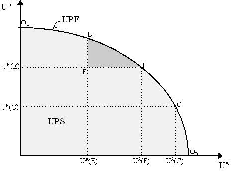
However, many Paretians, as could be expected, were dissatisfied Robbins's conclusion and launched the "New Welfare Economics" movement in 1930s. New Welfare Economics accepted the argument that utility is not comparable across people, but nonetheless thought that welfare judgements could nonetheless be made by appropriate modifications of the concept of Pareto-optimality. We can divine two strains of New Welfare Economics, which we shall call the "Harvard" and the "L.S.E." positions, respectively. The "Harvard" position is associated mainly with Abram Bergson (1938) and Paul Samuelson (1938, 1947, 1950). Roughly, the Harvard position accepts that individual utilities are not comparable and also accepts Robbins's contention that the choice of social optimum is a normative issue. However, unlike Robbins, it does not accept that it lies outside the purview of economics. The "L.S.E." position, expounded by Nicholas Kaldor (1939), John Hicks (1939) and Tibor Scitovsky (1941), is a bit braver. Again, it accepts that individual utilities are not comparable, yet it does not regard social choice as a normative issue, but rather a clearly positive one. All that is necessary is to construct the proper criteria for comparison of social situations which does not involve value judgments of any sort, that one can make the same welfare conclusions regardless of whether "one is a liberal or a socialist, a nationalist or an internationalist, a christian or a pagan" (Hicks, 1939). (we should note that Scitovsky (1951) is much more restrained in his claims). However, the utilitarianian did not just evaporate and die but were given a new coat a point and relabeled as the "Distributists". Ian M.D. Little (1949, 1950) led the charge against New Welfare Economics. Specifically, Little argued that individual utilities are comparable in a scientific manner, and thus the choice of social optimum is a positive issue which economists should, indeed must, analyze. As he writes, "interpersonal comparisons of satisfaction are empirical judgments about the real world, and are not, in any normal context, value judgments" (Little, 1950: p.66). Little's basic argument, reiterated by Dennis H. Robertson (1950, 1951), is almost "behaviorist" in tone. We need not worry so much about "utility and all that" but concentrate instead on things we can empirically see, such as people's reactions to income. We can safely say that a dollar to a poor man means more than a dollar to rich man. This does not rely on "interpersonal comparisons of utility" in a formal sense, but it is plain common sense, i.e. an empirically-validated hypothesis. We should also mention that the old utilitarian "stochastic argument" for equity, that had been forwarded earlier by Edgeworth (1877, 1881), was reiterated by Abba P. Lerner (1944: p.24-32). Admittedly, Lerner argued, we do not know what people's "capacities for satisfaction" are, and thus we have no way of compare the utility gains of one person with the utility losses of another from a proposed policy. However, the statistical expression for the term "we do not know" translates itself into saying that every alternative is equally likely. This is Laplace's principle of indifference. Consequently, as we do not have any reason to assume Mr. A has a greater capacity for satisfaction than Mrs. B, then we can do no better than to assume they have equal capacities for satisfaction. It is in this manner, then, that Lerner drives us right back into the arms of Pigouvian welfare theory and his famous result that "if it is desired to maximize the total satisfaction in a society, the rational procedure is to divide income on an egalitarian basis" (Lerner, 1944: p.32). [for a critique of Lerner, see Milton Friedman (1947)]. Finally, we should mention that the Oskar Lange (1936, 1938) and Abba Lerner (1934) also resurrected the old Pareto-Barone position on the efficiency of a socialist society -- thus reigniting the "Socialist Calculation debate" with the Austrian economists. Roughly speaking, the Robbinsian, the Harvard, the LSE and the Distributist positions were the four sides involved in the debate over the New Welfare Economics that raged for over a decade in the 1940s, a debate whose terms and tone changed considerably after Kenneth J. Arrow's famous "Impossibility Theorem" (Arrow, 1951). We take up first the L.S.E. theory, and consider the Harvard theory later. We treat Arrow's theory elsewhere. (A) Utility Possibilities Frontiers Although Vilfredo Pareto (1906) introduced the Edgeworth-Bowley box, "Pareto's economics would have been better understood had he explicitly used the utility frontier concept" (Samuelson, 1962). The "utility possibilities frontier" (UPF) and the "grand utility possibilities frontier" (GUPF) were introduced into economics by Maurice Allais (1943), who originally called it the "surface de rendement maximum" (Allais, 1943: p.641) and, later, renamed it the "surface d'efficacité maximum" (Allais, 1989: p.45). Independently of Allais, Paul Samuelson (1947: p.244) hinted at a "possibility function" and finally drew a utility possibility frontier explicitly in Samuelson (1950). The utility possibilities frontier (UPF) is the upper frontier of the utility possibilities set (UPS). The UPS is the set of utility levels of agents possible for a given amount of output, and thus the utility levels possible in a given consumer Edgeworth-Bowley box. This is drawn in Figure 1 below for the two agent case. The UPF itself is the contract curve of the Edgeworth-Bowley box. The extremes of the UPF represent the utilities of the agents at the origins of the Edgeworth-Bowley box: OA (where A has her minimum utility and B his maximum) and OB (where A has maximum utility, and B his minimum). The points C, D and E in the Edgeworth-Bowley box we constructed earlier in Figure 2 of the Paretian System I, are now represented by their equivalent points in Figure 1 below.
Recall that at point E in the Edgeworth-Bowley box, we had a "lens" formed by the indifference curves representing utility levels UA(E) and UB(E). This is the "distributable surplus" as Allais (1943, 1989) named it, perhaps better known as the set of allocations that are Pareto-superior to E. This "lens" is now the shaded are in Figure 1. Points C, D and F represent points of tangency of the utilities, thus they are all on the contract curve and thus all on the utility possibilities frontier (UPF). As it happens, the UPF is drawn in this diagram as a concave function but this is not necessarily the case. Concavity of the UPF will only be true if we have cardinal utilities which are comparable across agents and this assumption ought not to be made. In general, the UPF is neither concave nor convex but only needs to be downward sloping. Nonetheless, we can still derive the slope of the UPF at any point. To see this, recall that as the UPF represents the contract curve of an Edgeworth-Bowley box, then everywhere along it, MRSAXY = MRSBXY. The slope of the UPF represents the gain in utility of one agent relative to the loss in utility of the other agent by a marginal reallocation of outputs. Thus, we can take amount dX from agent A and give it to B. Now, given utility functions UA(X, Y) and UB(X, Y), then we know that, by total differentiation:
which indicates the change in utilities that arise by transferring dX from A to B. Recall that Uhi is the marginal utility of good i for household h. Thus, rearranging, we see that:
Thus, as the MRSs must be equal along the UPF, which implies, after some rearrangement, that:
so the slope of the UPF is equal to the negative of the ratios of marginal utilities of good Y for both agents. Now, recall from the first order conditions for a utility-maximization problem that UAY - m ApY = 0 and UBY - m BpY = 0 where Lagrangian multipliers m A and m B are the marginal utilities of income for agents A and B respectively. Thus, we can see from this that UBY/UAY = m B/m A, or, plugging into our earlier equation:
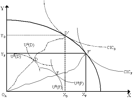
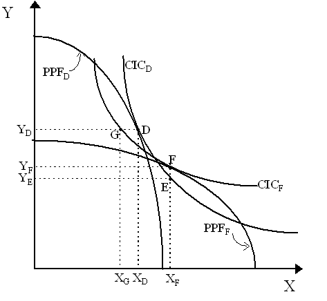
thus, the slope of the UPF is equal to the negative of the ratio of marginal utilities of income. If we assume cardinal utilities which are comparable, then the UPF will have a concave shape as in Figure 1 representing the principle of diminishing marginal utility - as we move down the UPF from OA to OB by allocating output from B to A along the contract curve, we are increasing the utility of agent A and decreasing that of B. The principle of diminishing marginal utility then applies, as this implies m B/m A increases in the move from OA to OB, so the slope of the UPF becomes more negative. However, while the UPF may be adequate for pure exchange economies, it clearly will not do for production economies. As shown in Figure 2, allocations D and F are both Pareto-optimal allocations in an economy with production. Yet, D and F arise in different Edgeworth-Bowley boxes defined by different output combinations (XD, YD) and (XF, YF). As a UPF is derived only for a single Edgeworth-Bowley box, most of the allocations on the contract curve within a particular box - and thus most points on a particular UPF - are not Pareto-optimal allocations at all when production is considered. For instance, as we saw earlier in Figure 5 in our discussion of the Paretian System II, at a particular point on the contract curve, the MRSs will be equal, but it is not necessarily the case that it will also be that MRSXY = MRPTXY (tangency of CIC and PPF). In fact, as Figure 2 shows, usually only one or perhaps a few of the points on the contract curve of a particular consumer Edgeworth-Bowley box will correspond properly to Pareto-optimal allocations in a production economy - i.e. those allocations which also yield a tangency between the corresponding CICs and the PPF.
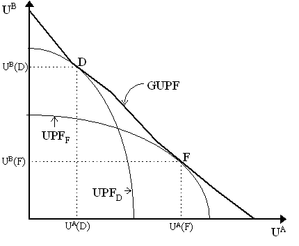
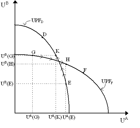
To obtain the analogue of a UPF for a production economy, we need to construct a "grand utility possibilities frontier" (GUPF) as shown in Figure 3 as the envelope of a series of UPFs. In Figure 3, UPFF corresponds to the contract curve obtained from the Edgeworth-Bowley box defined by output allocation F¢ in Figure 2. Similarly, UPFD corresponds to the contract curve in the Edgeworth-Bowley box defined by output allocation D¢ in Figure 3. Point F on the UPFF and point D on UPFD correspond to the utility combinations at points D and F in Figure 2. Thus, only D and F in Figure 3 are actually Pareto-optimal allocations (i.e. that yield tangencies between CICD and CICF to the PPF in Figure 2), the rest of the utility combinations on UPFC and UPFD, although they represent points on the respective contract curves, they are not themselves Pareto-optimal as they do not fulfill the CIC-PPF tangency conditions.
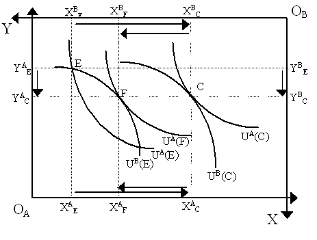
As every output allocation yields different UPFs, then we can draw a series of them and thereby construct the GUPF as the envelope of the UPFs which passes through the proper Pareto-optimal allocations D, F and so on. Thus, every point on the GUPF actually corresponds to Pareto-optimal allocations in a production economy. Consequently, points in the interior of the GUPF are necessarily Pareto-suboptimal points and thus the "distributable surplus" from a Pareto-suboptimal point is represented by the set to the northeast of that point up to the GUPF. Utility combinations above the GUPF are, of course, unattainable. [Note: our UPF and GUPF are in the literature following Samuelson (1950) sometimes referred to as the "utility possibilities curve" (UPC) and "utility possibilities frontier" (UPF) respectively. As it is often confusing to differentiate between curves and frontiers (and as in a pure exchange economy, they are the same), we adhere to calling everything a "utility possibilities frontier" and allow our modifier, "grand" differentiate between the pure exchange and production economy case]. As noted, the L.S.E. position argued that individual utilities are not comparable, but that nonetheless that does not imply that choosing some Pareto-optimal allocations over other Pareto-optimal allocations is a "normative" concern. Rather, there are some "objective" criteria for ranking allocations which, if followed consistently, would lead to social improvements. The only welfare criteria we have considered, thus far, has been Pareto-optimality. To this, the L.S.E. economists, in particular Nicholas Kaldor, John Hicks and Tibor Scitovsky, launched a search for another criteria which could be deemed "objective". In a pure exchange Edgeworth-Bowley box in Figure 4 below, we see that the allocations D and F (and indeed, all allocations in the "lens" formed by UA(E) and UB(E)) are Pareto-superior to E, but allocation C cannot be compared to either D, F or E. These points are compatible with the points in the UPF shown in Figure 1 above. An alternative criteria of judging whether an allocation was "preferable" to another was proposed by Nicholas Kaldor (1939). Effectively, he argued that an allocation is preferred to another allocation if by moving from the second to the first, the "gainer" from the move can, by a lump-sum transfer, compensate the "loser" for his loss of utility and still make a gain in utility for herself. This idea had already been intimated by Enrico Barone (1908) and Jacob Viner (1937: p.533-4). We can see the Kaldor compensation criteria in Figure 4 below. Suppose we propose to move from allocation E to allocation C. Obviously, agent A gains in utility (from UA(E) to UA(C)) and agent B loses (from UB(E) to UB(C)) - thus E and C are not Pareto-comparable. Nonetheless, if we move to allocation C, agent A can pay agent B a portion of her gains so as the keep agent B at his old utility level UB(E). For instance, A can pay B the amount XAC - XAF (thus we move to point F) so that B retains the same old utility level UB(E) while the utility of A is now UA(F). As XAC > XAF, then agent A makes a net gain of XAE + (XAC - XAF) plus whatever she gained in terms of good Y. Thus, as we see in Figure 1, as UA(F) > UA(E), it is worthwhile for her to propose moving to C and then paying agent A the amount XAC - XAF, thereby moving the economy to F.
Now, if the Kaldor compensation criteria implied merely that we moved from E to F, then it is not an improvement on the Pareto criterion as F is obviously Pareto-superior to E. However, Kaldor's innovation is to propose that allocation C is superior to allocation E because it is possible for A to compensate B and still be better off. The crucial point is that A can compensate B, and not that A will compensate B. Thus, the move from E to C is actual, but the move from C to F is only hypothetical. Thus, Kaldor proposed that we can compare Pareto-incomparable points via this "hypothetical compensation" test: in sum, an allocation is preferable to another if it is possible to hypothetically redistribute goods so that a Pareto-improvement occurs. While the Kaldor criteria can be used to compare Pareto sub-optimal points with each other and with Pareto-optimal points, the Kaldor criteria remains incomplete because it cannot compare Pareto-optimal points to each other: e.g. a movement from Pareto-optimal allocation to another Pareto-optimal allocation (e.g. C and F in Figure 4) will require, via compensation, that the winning agent surrender all his gains - thus she will be not be better off. An alternative test, proposed by John Hicks (1939, 1940) was that of "bribery" by the losers as opposed to "compensation" by the winners. An allocation would be preferable to another if, given a proposed move from the second to the first, the losers would not be able to bribe the winners into not undertaking the move. If they were willing to give such a bribe and the winners were willing to take it instead of moving to the proposed allocation, then the proposed state would not be superior. Thus, in the case of Figure 4, we might think that agent B might offer agent A a bribe not to move from allocation E to allocation C, but clearly A would not accept. There is thus, from E, no lump-sum transfer that agent B would be willing to give agent A that would make A no worse off than in state C. As a consequence, C is preferred to E by the Hicks criteria. Conceptually, then, the Hicks criteria reverts the Kaldorian notion: C is preferred to E if from E it is not possible to undertake a hypothetical lump-sum redistribution to achieve a Pareto-improvement over state C. To capture the Kaldor-Hicks criteria in a production economy, we now need to consider it in reference to the GUPF and the allocational possibilities within them. Thus, an allocation is superior to another allocation if it is possible that the winners compensate the losers for moving to the former (Kaldor) or if the losers bribe the winners not to move to the former (Hicks). In a production context, there are now two forms of the Kaldor criteria:
It is clear that the weak Kaldor criteria can compare all Pareto-suboptimal points in the GUPF. However, the strong Kaldor criteria cannot compare all suboptimal points in the GUPF. This is the complication that production begins into the story. To see this more clearly, consider Figure 5, where we have drawn two UPF's. Suppose we wish to compare points E and G. Obviously, E is Pareto-inferior to F and G is Pareto-inferior to D, but it is not possible to compare E and G by the Pareto criterion. Let us then employ the strong Kaldor compensation test: if we move from point E to point G, it is obvious that agent B is the winner and agent A is the loser. However, B can (hypothetically) compensate A for his loss and still remain better off by offering a compensation that takes the allocation to point H (note that both G and H are on the same frontier, UPFF - this is the requirement of the strong Kaldor criteria). At H, agent A would be at his old utility level, UA(E), but agent B would have utility UB(H) > UB(E), thus she is strictly better off. Thus, by the Kaldor compensation criteria, allocation G is superior to allocation E.
However, consider now the following: suppose we begin at G and propose a move towards E. Agent A is now the winner and B the loser. Yet, agent A can hypothetically compensate agent B by offering a transfer payment that takes the allocation to point K. At K, agent B stays at her old utility level UB(G), but agent A improves in utility from UA(G) to UA(K). Thus, by the strong Kaldor compensation criteria, E is superior to G. Thus, by the Kaldor strong criteria, E is superior to G and, by the same criteria, G is superior to E. Points E and G are not consistently comparable. (C) Scitovsky Reversals and the Double Criteria Granted that the strong Kaldor criteria is lacking in its ability to compare allocations, problems also arise with the weak Kaldor criteria for comparisons of welfare under different types of change. The famous Scitovsky reversal paradox, first identified by Tibor Scitovsky (1941), uncovered an important drawback of the weak Kaldor criterion. Suppose we are in a production economy and suddenly the production conditions change so that, as in Figure 6 below, we move from PPFD to PPFF. In order to judge whether this technological change improved or worsened welfare, we should attempt to compare the corresponding Pareto-optimal points D and F represented by the tangencies of CICD with PPFD and CICF with PPFF.
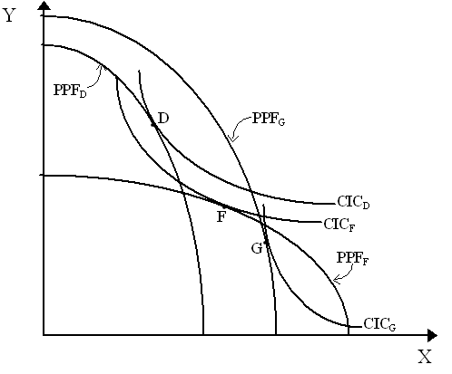
However, notice that CICD and CICF intersect each other. Specifically, recall that intersecting CICs imply Pareto-improvements: note that F is Pareto-superior to E and E, of course, represents the same level of "aggregate" utility as D as it lies on CICD (compare with the movement in Figure 1 above). Thus, from D, it is possible to hypothetically redistribute goods and outputs so that we obtain a Pareto-improvement. Thus, according to the weak Kaldor criteria, situation F is superior to D. However, by a reverse argument, we can note that moving from PPFF to PPFD, we can see that D is Pareto-superior to G and G yields the same level of "aggregate" utility as F as it lies on CICF. Thus, by the weak Kaldor criteria again, situation D is ranked higher than situation F. Thus, there is a "reversal" of rankings between D and F by the weak Kaldor criteria as F is better than D and D is better than F. Scitovsky (1941) suggested that the resolution to this reversal paradox might be combining both the Hicks and Kaldor criteria. Notice that the movement from D to F fulfills the Kaldor criteria but not the Hicksian one as, from D, it is possible to undertake a hypothetical lump-sum redistribution within PPFD that achieves a Pareto-improvement over F (e.g. a point slightly above G in PPFD is a Pareto-improvement over G and thus over F). Thus, the Scitovky double criteria states that an allocation is preferred to another if it fulfills both the Kaldor and Hicks criteria. This would, it seems, eliminate Scitovsky reversals as that depicted in Figure 6 above. However, as William Gorman (1955) demonstrated, while the Scitovsky double criteria rules out Scitovsky reversals, it does not rule out intransitive chains: for instance, it may be that an allocation G is preferred to allocation D, allocation D is preferred to allocation F but allocation F is not preferred to allocation G. This is shown in Figure 7, where we have three PPFs (PPFD, PPFF and PPFG) and three CICs corresponding to the Pareto-optimal allocations on each PPF (allocation D on CICD, allocation F on PPFF and allocation G on PPFG). Notice that unlike in Figure 6, D is superior to F by the Scitovsky double criteria because D is better than F by both the Kaldor and Hicks criteria (notice that CICD does not intersect PPFF while CICF intersects PPFD).
The problem of intransitivity can now be visualized in Figure 7. As noted, by the double criteria, D is preferred to F. By the same double criteria, G is preferred to D (as CICD intersects PPFG but CICG does not intersect PPFD). However, obviously G and D do not fulfill the double criteria (as CICF intersects PPFG and CICG intersects PPFF, a situation analogous to the one earlier in Figure 6). Thus, by the Scitovsky double criteria, G is preferred to D, D is preferred to F but G is not preferred to F. Thus although the Scitovsky double criteria rules out ranking reversals (note that although G is not preferred to F, F is also not preferred to G - they are merely incomparable), the ranking is intransitive. A way out of Gorman's intransitivity problem lies in the criteria proposed by Paul Samuelson (1950). The Samuelson criteria argues that a state G is preferred to a state D if all hypothetical redistributions from state G will achieve utility allocations that are superior to some hypothetical redistributions from state D and that no hypothetical redistribution from state D will yield utility allocations that are unattainable via hypothetical redistributions from state G. What this implies, of course, is that, utility space, that UPFG lies everywhere above UPFD. In production space, it requires that PPFG intersect the interior of CICD and the interior of any other CIC tangent to PPFD (notice the heavy information requirement that we know the CICs of all hypothetical reallocations). Clearly, this will often require that PPFG lies everywhere above PPFD - as in Figure 7. Naturally, if we deal exclusively with PPFs of this type, neither Scitovsky reversals nor Gorman intransitivities arise, but it also obviously highly restrictive as it rules out quite reasonable situations (e.g. those depicted in Figures 6 and 7). Thus, in this sense, the Samuelson criteria is far more restrictive than the Kaldor, Hicks or Scitovsky double criteria. In sum, disregarding the problems inherent in the Kaldor, Hicks and Scitovsky criteria, the question must be raised again: are these objective criteria in any sense? Ethically, of course, the Kaldor criteria is easily disputed as it is only a "could" and not a "would" or even a "should". As Ian M.D. Little writes, in his famous critique:
A point reiterated by many contemporaries (e.g. Baumol, 1946; Reder, 1947; Samuelson, 1947). There were three lines of defense followed by the L.S.E. economists. The first was to agree and make the "could" into a "would", i.e. have the winners actually compensate the losers. This, of course, leads to an improvements of sorts, the practical objection that arises is that once we are at a new allocation, winners are unlikely to surrender any of their gains. The second defense, pursued by Hicks (1941), was that even if the losers do not get compensated in the move, they might still benefit in the "long-run" if the criteria were followed consistently by society. This argument is similar to that of "trickle-down" theory and in arguments for free trade: some people may be worse off in the short-run, but in the long run, everyone will be better off. The underlying assumption, of course, is that at some point, those who lost utility initially will come across a possible move in which they benefit and a society which follows the Kaldorian rule will move to it and thus they will gain in the end. Of course, as Little (1950) notes, this is completely hypothetical. There is nothing to guarantee that there will eventually be a move in which the initial losers will be the ultimate winners. The third (and perhaps best) line of defense is that the Kaldor-Hicks criteria merely lay out what is economically possible and that it is up to policy-makers, on the basis of their own value judgements, to choose which move to make and whether compensation of the losers should be forced (cf. Kaldor, 1939; Scitovsky, 1951). Thus, they argue, they are merely underlining that certain options may be more economically possible than others, but they are still only options. The final decision will require more philosophical, ethical and political considerations to be brought into the story. (4) Bergson-Samuelson Social Welfare Functions What might be these philosophical considerations? Here we enter the normative side of things -- which, as the Harvard view argued -- is an inextricable part of the "New Welfare Economics". The great Harvard tool was the social welfare function introduced by Abram Bergson (1938). This unabashedly normative approach was followed by Bergson (1948, 1954), Paul Samuelson (1947, 1950, 1956), Gerhard Tintner (1946) and Jan de Van Graaff (1957). What has become known as the "Bergson-Samuelson" social welfare function (SWF) takes the following general form:
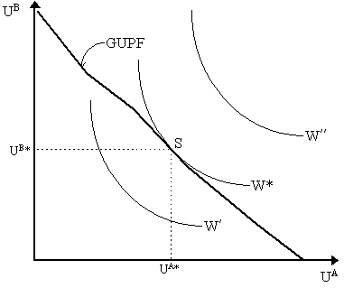
so that "society's" welfare denoted, W, is merely a function of the utilities of its constituent members, Uh, h = 1, 2, .., H, where H are the number of households in society. [This is what Amartya Sen (1977) later called a "welfarist" social welfare function in that society's welfare is dependent wholly on the utility of households and not, say, on the quantities of goods involved]. The purpose of the Bergson-Samuelson SWF can be envisaged in the context of grand utility possibilities frontier developed earlier (GUPF). Recall that every point on the GUPF is a Pareto-optimal allocation, and thus it seems that no point is necessarily preferable to another. The underlying objective of the Kaldor-Hicks-Scitovsky exercises were attempts to make these points comparable, presumably so a society could "rank" points in the utility space according to some acceptable form of social desirability. However, as noted earlier, the criteria could not really achieve such a ranking of Pareto-optimal points. The Bergson-Samuelson SWF had a more precise purpose in mind: given the set of Pareto-optimal points, which is more desirable from "society's" point of view, where the notion of social desirability was subsumed in a social welfare function. Heuristically, we can envisage the upper contour set of the SWF as a set of "social indifference curves" in utilities space, as shown in Figure 8. According to Bergson (1938), there are some desirable properties of a society which are captured by the SWF: for instance, that social welfare increases if the utility of any of its members increase and none decrease (the "Pareto principle") - that yields northeasterly ascendance of the social indifference curves. One might argue that equity is socially desirable, thus extreme distributions of utility ought to be given less weight, thus the convexity of the social indifference curves; we would like them to be non-intersecting, etc.
Reasoning along these lines, by superimposing social indifference curves on the GUPF as in Figure 8, we can see that allocation S = (UA*, UB*) is the point on the GUPF that attains the highest social indifference curve, and thus, in principle, maximizes the social welfare function, yielding social welfare index W*. Thus, the "social optimum" is determined by the tangency of the social indifference curves and the GUPF. It is a simple matter to derive the fact that the slope of the social indifference curves have slope is equal to the negative of (¶ W/¶ UA)/(¶ W/¶ UB). This last term is often denoted as the "marginal rate of social substitution" between agents A and B, or MRSSAB. Now, recall that the slope of the GUPF will be merely the ratios of the marginal utilities of income of agents A and B, thus the tangency condition is that:
thus, (¶ W/¶ UA)/m A = (¶ W/¶ UB)/m B, or the social marginal utility for each household is equal across households. There are several alternative types of social welfare functions. The one depicted above in Figure 8 can be captured by the following functional form:
where a h are the weights assigned to each household in the social welfare function. Such a function yield the convex social indifference curves in Figure 8 and is sometimes called a "Bernoulli-Nash" social welfare function. A more strictly Benthamite or "utilitarian" social welfare function would construct the SWF as a linear sum of weighted utilities, e.g.
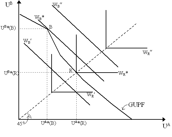
which is a direct sum. Thus, as stipulated by Jeremy Bentham (1789) and the utilitarians, this one maximizes the (weighted) sum of individual utilities and thus yields linear social indifference curves (WB¢ , WB*, WB¢¢ ) , as we see in Figure 9 below.
Another popular form is the "Rawlsian" or "maximin" social welfare function:
which seeks to maximize the utility of society's least happy member, as argued by the philosopher John Rawls (1971). This yields Leontief-type social indifference curves. Rawlsian social indifference curves are also depicted depicted in Figure 9. Notice that the Rawlsian structure implies a strictly egalitarian solution for the social optimum: as it ascends along the 45° ray (WR¢ , WR*, WR¢¢ ) in Figure 9, the social optimum (R) is always one of absolute equality of utility (UA*(R) = UB*(R)). In contrast, the Benthamite social welfare function yields a social optima (B) that can be quite unequal (UA*(B) < UB*(B)), as we see in Figure 9. It is worthwhile entertaining a Bergson-Samuelson SWF on the basis that one can obtain the conditions for "social justice", namely that:
so that the marginal rate of social substitution between agents A and B is equal to the ratio of marginal rates of substitution of A and B. What this implies is that the allocation of goods is such that the utility distribution is compatible with the "worthiness" of the individuals according to the social welfare function. This condition is obtainable in general via an exercise akin to that of Oskar Lange (1942) and Maurice Allais (1943), except that instead of maximizing a single individual's utility subject to the constraint that all others are at a given utility level, we just maximize the social welfare function. Thus, in an economy with H individuals, F firms, n goods and m factors, we now have the following maximization problem:
Setting up a Lagrangian and deriving first order conditions, we obtain exactly the same results we had for the earlier Lange-Allais exercise with one difference: instead of having household multipliers, m h, we now replace that with ¶ W/¶ Uh. Thus, for instance, for every good, we now have:
and for every factor:
Combining, we still obtain the results that MRSAXY = MRSBXY = MRPTXY, etc. What we get extra is that, for any two households A, B = 1, .., H, we now have, combining the first order conditions for the ith good:
Thus:
which is our "social justice" condition. We shall avoid going into any details here on the construction of social welfare functions from social preference orderings (and, in turn, from individual preference orderings, the main exercise of Arrow (1951)), which is quite a large and self-contained field. Finally, we should note that few of the New Welfare Economists said anything about the implementation of the social plan once one is chosen. This would bring in the type of public choice concerns of economists such as Frank H. Knight and James M. Buchanan. The main implications here is that when social choice and implementation are considered together, the social optimum may turn out to be quite different. _________________________________________________________________ M. Allais (1943) Traité d'Economie Pure, 1952 edition of A la Recherche d'une Discipline Economique, Paris: Impremerie Internationale. M.Allais (1989) La Théorie Générale des Surplus. Grenoble: Presses Universitaires de Grenoble. Originally published in Économies et Sociétés, 1981, Nos. 1-5. K.J. Arrow (1951) Social Choice and Individual Values. 1963 edition, New Haven: Yale University Press. E. Barone (1908) "The Ministry of Production in the Collectivist State", Giornale degli Economisti, as translated in Hayek, 1935, editor, Collectivist Economic Planning, London: Routledge. W.J. Baumol (1946) "Community Indifference Curves", Review of Economic Studies, Vol. 14 (1), p.44- J. Bentham (1789) Introduction to the Principles of Morals and Legislation. London: Athlone. A. Bergson (Burk) (1938) "A Reformulation of Certain Aspects of Welfare Economics", Quarterly Journal of Economics, Vol. 52, p.310-34. A. Bergson (1954) "On the Concept of Social Welfare", Quarterly Journal of Economics. K.E. Boulding (1952) "Welfare Economics", in Haley, editor, Surveys of Contemporary Economics, Vol. II Homewood, Ill: Irwin. J.S. Chipman and J.C. Moore (1978) "The New Welfare Economics, 1939-1974", International Economic Review, Vol. 19, p.547-84. F.Y. Edgeworth (1881) Mathematical Psychics: An essay on the application of mathematics to the moral sciences. 1961 reprint, New York: Augustus M. Kelley. F.Y. Edgeworth (1925) Papers Relating to Political Economy, 3 volumes, London: Macmillan. M. Friedman (1947) "Lerner on the Economics of Control", Journal of Political Economy, Vol. 55, p.405-16. J. de Van Graaff (1957) Theoretical Welfare Economics. Cambridge, UK: Cambridge University Press. W.M. Gorman (1955) "The Intransitivity of Certain Criteria Used in Welfare Economics", Oxford Economic Papers, Vol. 7, p.25-35. H.H. Gossen (1854) The Laws of Human Relations and the Rules of Human Action Derived Therefrom. 1984 translation, Cambridge, Mass: M.I.T. Press. R.F. Harrod (1938) "The Scope and Method of Economics", Economic Journal, Vol. 68, p.389-97. J. Hicks (1939) "The Foundations of Welfare Economics", Economic Journal, Vol. 69, p.696-712. J. Hicks (1940) "The Valuation of Social Income", Economica, Vol. 7, p.105-24. J. Hicks (1941) "The Rehabilitation of Consumer's Surplus", Review of Economic Studies, Vol. 8, p.108-16. J. Hicks (1975) "The Scope and Status of Welfare Economics", Oxford Economics Papers, Vol. 27 (3), p.307-26. N. Kaldor (1939) "Welfare Propositions in Economics and Interpersonal Comparisons of Utility", Economic Journal, Vol. 69, p.549-52. O. Lange (1942) "The Foundations of Welfare Economics", Econometrica, Vol. 10 (3), p.215-28. C.W.F. Launhardt (1885) Mathematische Begründung der Volkwirtschaftslehre. Leipzig: Engelmann. A.P. Lerner (1944) The Economics of Control: Principles of welfare economics. New York: Macmillan. I.M.D. Little (1949) "The Foundations of Welfare Economics", Oxford Economic Papers, Vol. 1, p.237-8. I. M.D. Little (1950) A Critique of Welfare Economics. 1957 edition, Oxford, UK: Oxford University Press. E.J. Mishan (1960) "A Survey of Welfare Economics, 1939-59", Economic Journal, Vol. 7, p.197-265. V. Pareto (1896-8) Cours d'économie politique. 2 volumes. 1964 edition, Geneva: Librairie Droz. V. Pareto (1906) Manual of Political Economy. 1971 translation of 1927 edition, New York: Augustus M. Kelley. A.C. Pigou (1912) Wealth and Welfare. 1920 edition, The Economics of Welfare. London: Macmillan. J. Rawls (1971) A Theory of Justice. Cambridge, Mass: Harvard University Press. M.W. Reder (1947) Studies in the Theory of Welfare Economics. Oxford: Oxford University Press. L.C. Robbins (1932) An Essay on the Nature and Significance of Economic Science. 1984 edition, New York: New York University Press. L.C. Robbins (1938) "Interpersonal Comparisons of Utility: A comment", Economic Journal, Vol. 48, p.635-41. L.C. Robbins (1981) "Economics and Political Economy", American Economic Review, Vol. 71 (2), p. D.H. Robertson (1950) "A Revolutionist's Handbook", Quarterly Journal of Economics, Vol. ??, p. D.H. Robertson (1951) "Utility and All That", Manchester School. P. A. Samuelson (1938) "Welfare and International Trade" , American Economic Review, Vol. 28, p.261-6. P.A. Samuelson (1947) Foundations of Economic Analysis. 1983 edition. Cambridge, Mass: Harvard University Press. P.A. Samuelson (1950) "Evaluation of Real National Income", Oxford Economic Papers, Vol. 2, p.1-29. P.A. Samuelson (1956) "Social Indifference Curves", Quarterly Journal of Economics, Vol. 70, p.1-22. T. Scitovsky (1941) "A Note on Welfare Propositions in Economics", Review of Economic Studies, Vol. 9, p.77-88. T. Scitovsky (1951) "The State of Welfare Economics", American Economic Review, Vol. 41, p.303- G. Tintner (1946) "A Note on Welfare Economics", Econometrica, Vol.14 , p.69-78. J. Viner (1937) Studies in the Theory of International Trade. New York: Harper. L. Walras (1874) Elements of Pure Economics: Or the theory of social wealth. 1954 translation of 1926 edition, Homewood, Ill.: Richard Irwin. L. Walras (1896) Etudes d'économie sociale: théorie de la répartition de la richesse sociale. 1990 Dockès edition, Paris: Economica. L. Walras (1898) Etudes d'économie politique appliquée: Theorie de la production de la richesse sociale. 1992 Potier edition, Paris: Economica. K. Wicksell (1893) Value, Capital and Rent. 1970 reprint of 1954 edition, New York: Augustus M. Kelley. K. Wicksell (1901) Lectures on Political Economy, Vol. 1. 1967 reprint of 1934 edition, New York: Augustus M. Kelley. K. Wicksell (1959) Selected Papers on Economic Theory, E. Lindhahl editor, R.S. Stedman translation, London: Allen & Unwin. _________________________________________________________________
|
All rights reserved, Gonçalo L. Fonseca
